As a part of the R4DS June Challenge and the “Summer of Data Science” Twitter initiative started by Data Science Renee, I decided to improve my text mining skills by working my way through Tidy Text Mining with R by Julia Silge and David Robinson. I wanted a fun dataset to use as I made my way through the book, so I decided to use every line from The Office. I could write an entire blog post about why I love The Office and why it is such a great show, but I will refrain. The good thing about using this dataset is that I’ve seen every episode (except for seasons 8 and 9) multiple times; needless to say, I know this data very well.
Let’s get started!

library(tidyverse)
library(tidytext)
library(scales)
library(googlesheets)
library(igraph)
library(ggraph)
library(widyr)
library(psych)
library(kableExtra)
library(knitr)
library(plotly)
library(ggcorrplot)
library(reticulate)
library(cleanNLP)
library(packcircles)
library(patchwork)
Getting and Cleaning the Data
Fortunately, someone created a googlesheet sourced from officequotes.net with every line from The Office.
# get key for data sheet
sheet_key <- gs_ls("the-office-lines") %>%
  pull(sheet_key)

# register sheet to access it
reg <- sheet_key %>%
  gs_key()

# read sheet data into R
raw_data <- reg %>%
gs_read(ws = "scripts")| id | season | episode | scene | line_text | speaker | deleted |
|---|---|---|---|---|---|---|
| 1 | 1 | 1 | 1 | All right Jim. Your quarterlies look very good. How are things at the library? | Michael | FALSE |
| 2 | 1 | 1 | 1 | Oh, I told you. I couldn’t close it. So… | Jim | FALSE |
| 3 | 1 | 1 | 1 | So you’ve come to the master for guidance? Is this what you’re saying, grasshopper? | Michael | FALSE |
| 4 | 1 | 1 | 1 | Actually, you called me in here, but yeah. | Jim | FALSE |
| 5 | 1 | 1 | 1 | All right. Well, let me show you how it’s done. | Michael | FALSE |
| 6 | 1 | 1 | 2 | [on the phone] Yes, I’d like to speak to your office manager, please. Yes, hello. This is Michael Scott. I am the Regional Manager of Dunder Mifflin Paper Products. Just wanted to talk to you manager-a-manger. [quick cut scene] All right. Done deal. Thank you very much, sir. You’re a gentleman and a scholar. Oh, I’m sorry. OK. I’m sorry. My mistake. [hangs up] That was a woman I was talking to, so… She had a very low voice. Probably a smoker, so… [Clears throat] So that’s the way it’s done. | Michael | FALSE |
This data, like the majority of data isn’t perfect, but it’s in pretty good shape. There are some clean up steps we need to do:
- Filter out deleted scenes
- Remove text in brackets ([]) and put in a new column called actions
- There are 4000+ instances of ??? found in the data mainly in the last two seasons. The ??? replaces … - ’ and “. For now I’m just going to replace all instances with ’ since that seems to be the majority of the cases
- Change speaker to lower case since there is some inconsistent capitalization
- Some entries for speakers have actions ([]), which I’ll remove
- Fix misspellings in the speaker field (e.g. Micheal instead of Michael)
mod_data <- raw_data %>%
  filter(deleted == "FALSE") %>%
  mutate(actions = str_extract_all(line_text, "\\[.*?\\]"),
         line_text_mod = str_trim(str_replace_all(line_text, "\\[.*?\\]", ""))) %>%
  mutate_at(vars(line_text_mod), funs(str_replace_all(., "���","'"))) %>%
  mutate_at(vars(speaker), funs(tolower)) %>%
  mutate_at(vars(speaker), funs(str_trim(str_replace_all(., "\\[.*?\\]", "")))) %>%
  mutate_at(vars(speaker), funs(str_replace_all(., "micheal|michel|michae$", "michael")))
Exploring the Data
total_episodes <- mod_data %>%
  unite(season_ep, season, episode, remove = FALSE) %>%
  summarise(num_episodes = n_distinct(season_ep)) %>%
  as.integer()

total_episodes
## [1] 186Searching around on the interwebs indicates that there were 201 episodes of the office, however the data I have contains 186 episodes. Wikipedia counts some episodes like “A Benihana Christmas” as two, but I’m not sure why. The data from officequotes.net closely matches the episode breakdown on IMdB with the exception of season 6. Officequotes.net counts Niagara parts 1 & 2 as one episode and The Delivery parts 1 & 2 as one episode instead of two. Since, I am working with the officequestions.net data, I’m going with the idea that there were 186 episodes total.
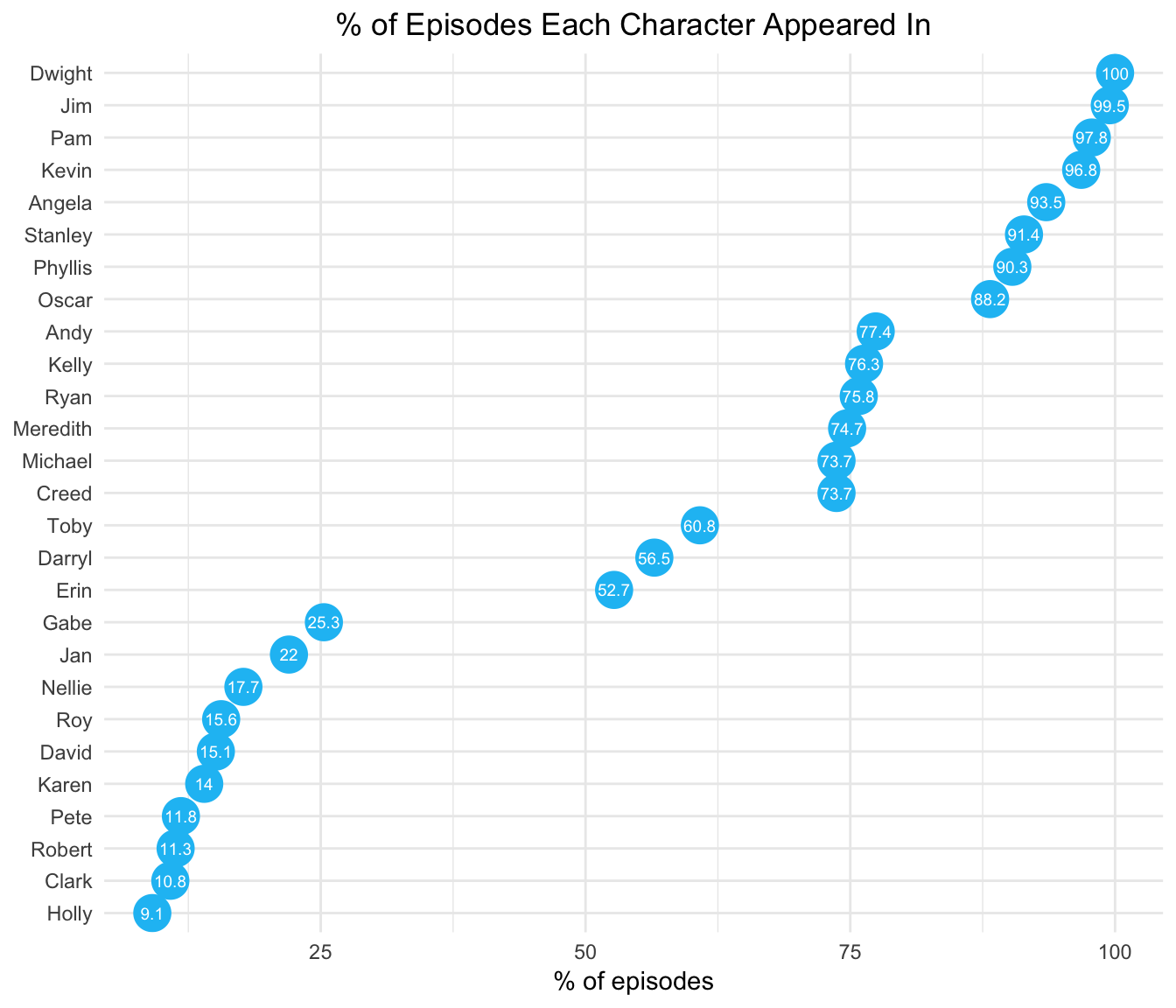
# proportion of episodes each character was in
episode_proportion <- mod_data %>%
  unite(season_ep, season, episode, remove = FALSE) %>%
  group_by(speaker) %>%
  summarise(num_episodes = n_distinct(season_ep)) %>%
  mutate(proportion = round((num_episodes / total_episodes) * 100, 1)) %>%
  arrange(desc(num_episodes))

total_scenes <- mod_data %>%
  unite(season_ep_scene, season, episode, scene, remove = FALSE) %>%
  summarise(num_scenes = n_distinct(season_ep_scene)) %>%
  as.integer()

# proportion of scenes each character was in
scene_proportion <- mod_data %>%
  unite(season_ep_scene, season, episode, scene, remove = FALSE) %>%
  group_by(speaker) %>%
  summarise(num_scenes = n_distinct(season_ep_scene)) %>%
  mutate(proportion = round((num_scenes / total_scenes) * 100, 1)) %>%
  arrange(desc(num_scenes))
Dwight was the only character in every episode.

Despite making only one appearance in the last two seasons of the show, Michael was still in the most scenes. 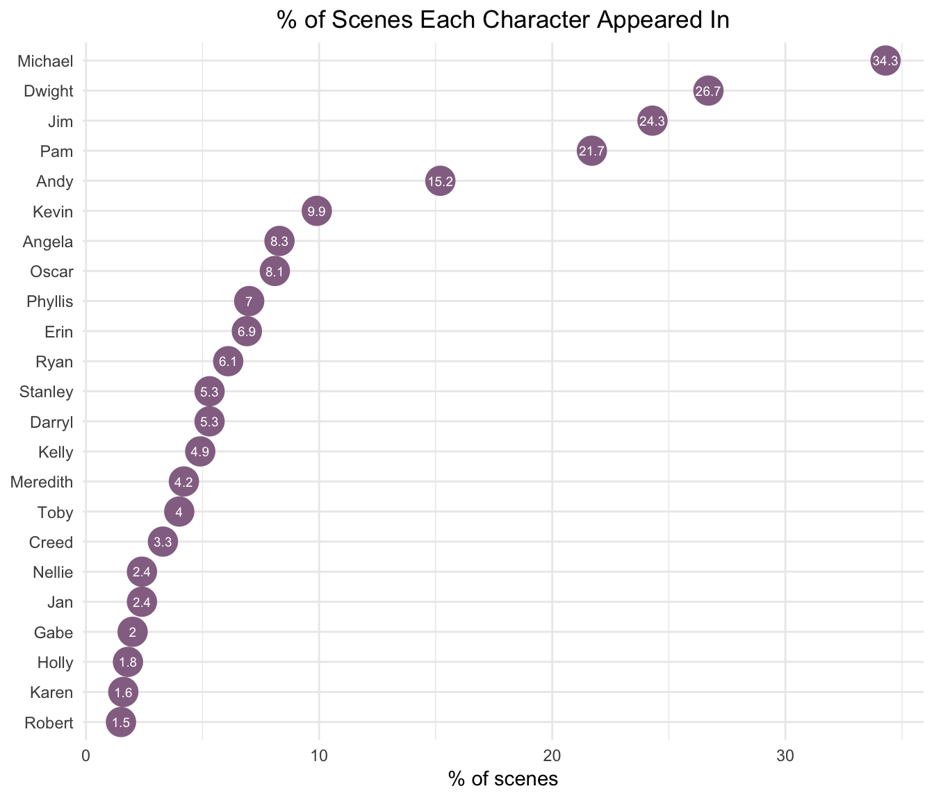
Determining the Main Characters
For parts of my analysis, I wanted to look at the main characters, but beyond Michael, Dwight, Jim, and Pam, determining who the “main characters” are is a little challenging. There are lots of ancillary characters that lurk in the background or get their own plot lines later in the show. I defined the main characters based on % of lines for the entire series. I included a character as a main character if they had at least 1% of all the lines. Yes, this excludes characters like Nellie and Robert California who played larger roles late in the series, but I wasn’t a big fan of those seasons, so it’s ok.
line_proportion <- mod_data %>%
  count(speaker) %>%
  mutate(proportion = round((n / sum(n)) * 100, 1)) %>%
  arrange(desc(n))

# define main characters based on line proportion
main_characters <- factor(line_proportion %>%
                            filter(proportion >= 1) %>%
                            pull(speaker) %>%
                            fct_inorder()
                          )
Now that we have the main characters defined, we can look at the the percent of lines each character had over the 9 seasons of the show.
line_proportion_by_season <- mod_data %>%
  group_by(season) %>%
  count(speaker) %>%
  mutate(proportion = round((n / sum(n)) * 100, 1)) %>%
  arrange(season, desc(proportion))

line_proportion_over_time <- line_proportion_by_season %>%
  filter(speaker %in% main_characters) %>%
  ggplot(aes(x = season, y = proportion, color = speaker, label = proportion)) +
  geom_point(size = 2) +
  geom_line() +
  scale_x_continuous(breaks = seq(1, 9, 1)) +
  theme_minimal() +
  theme(legend.position = "none") +
  labs(y = "% of lines",
       title = "% of Lines by Season") +
  theme(plot.title = element_text(hjust = 0.5)) +
  facet_wrap(~ factor(str_to_title(speaker), levels = str_to_title(main_characters)), ncol = 3) +
  geom_text(vjust = -1.2, size = 3.5) +
  ylim(0, 50) +
  scale_color_manual(values = office_colors)


line_proportion_over_time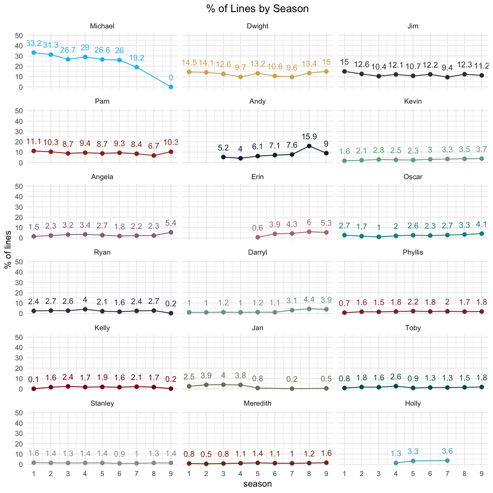
Text Analytics
Word Frequencies
I’ll start by tokenizing the text into words, removing the standard stop words (very common words that only add noise to the analysis), and plotting the most frequent words.
tidy_tokens <- mod_data %>%
  select(line = id, line_text_mod, everything(), -line_text, -actions, -deleted) %>%
  unnest_tokens(word, line_text_mod, strip_numeric = TRUE) %>%
  mutate_at(vars(word), funs(str_replace_all(., "'s$", "")))

tidy_tokens_no_stop <- tidy_tokens %>%
  anti_join(stop_words, by = "word")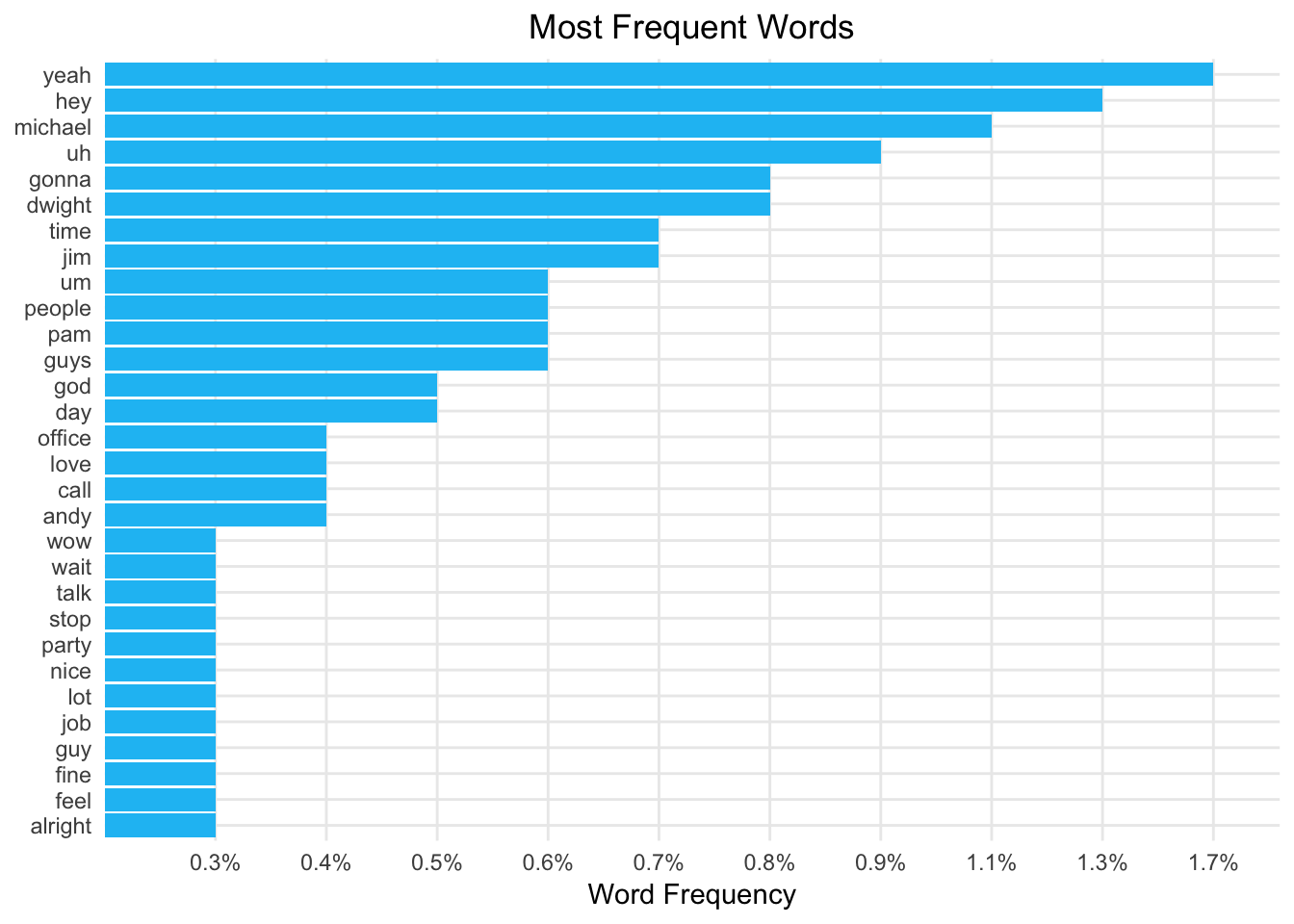
Looking at the most frequent words revealed words like “yeah”, “hey”, “uh”, “um”, “huh”, “hmm”, and “ah.” I’m going to add these to the stop words and remove them from the analysis.
custom_stop_words <- bind_rows(data_frame(word = c("yeah", "hey", "uh", "um", "huh", "hmm", "ah", "umm", "uhh", "gonna", "na", "ha", "gotta"),
                                          lexicon = c("custom")),
                               stop_words)

tidy_tokens_no_stop <- tidy_tokens %>%
  anti_join(custom_stop_words, by = "word")
After I removed those stop words, I was interested in looking at word frequencies by character.
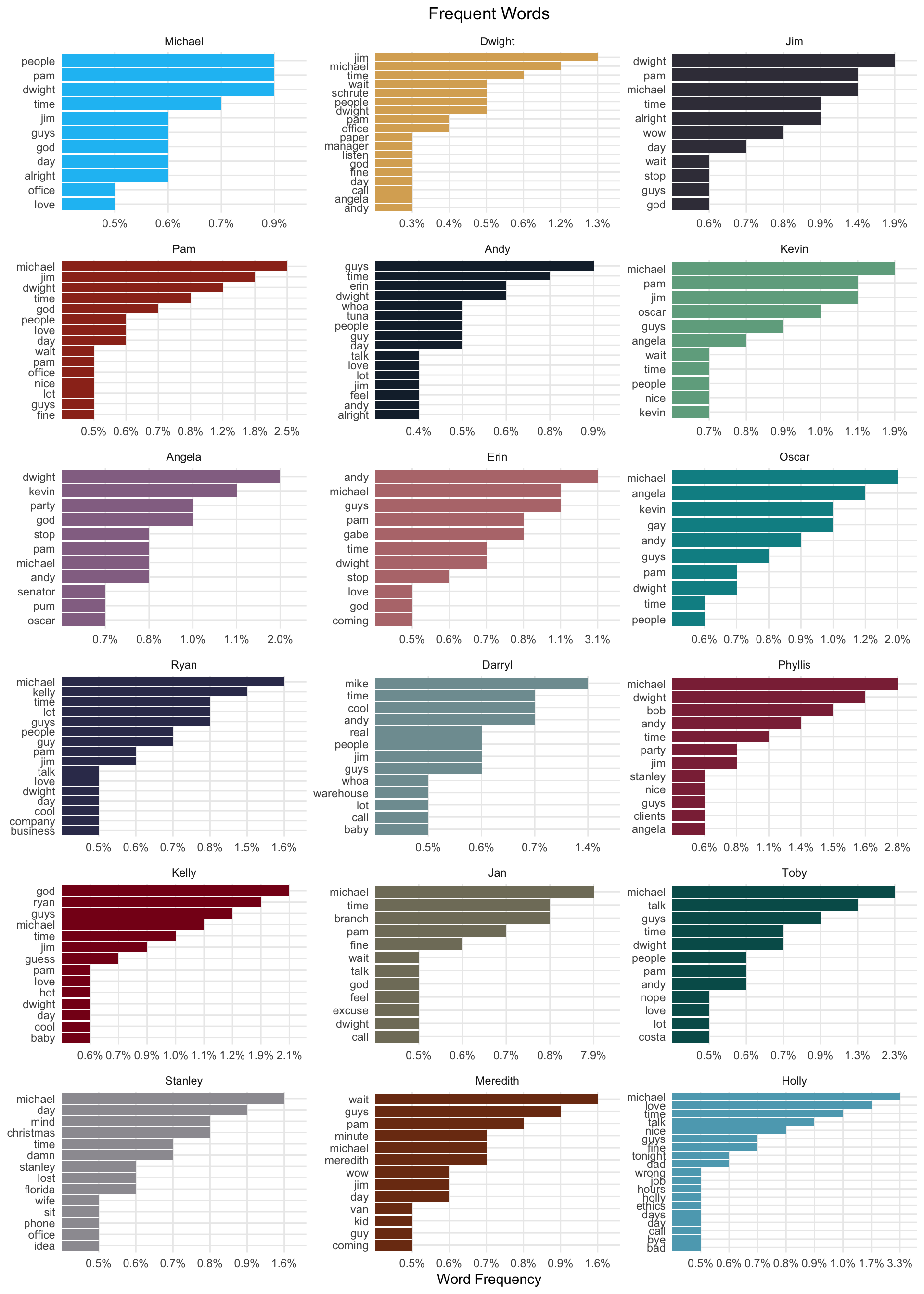
“Michael” is the most frequently used word for almost all of the characters. Given he is the main character and interacts with everyone that isn’t too surprising. A lot of characters use the words “time”, “god”, “guy(s)”, “love”, and “office” frequently. The word “party” is used frequently by Angela and Phyllis because they are on the party planning committee.

These word frequencies are interesting, but we see a lot of the same words used by different characters. If we want to understand the words that are unique to each character, we can use tf-idf. The tf-idf is defined as term frequency (tf) multiplied by inverse document frequency (idf). This gives us a measure of how unique a word is to a given character. Calculating tf-idf attempts to find the words that are important (i.e., common) for a given character, but not too common across all characters.
tidy_tokens_tf_idf <- tidy_tokens %>%
  count(speaker, word, sort = TRUE) %>%
  ungroup() %>%
  filter(speaker %in% main_characters) %>%
  bind_tf_idf(word, speaker, n)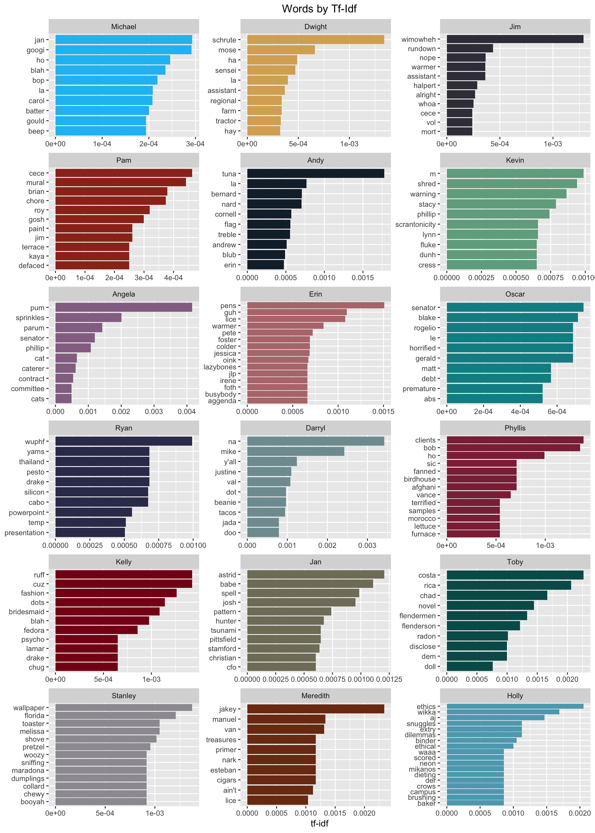
This is amazing and fun to see! There are so many good character nuances revealed. A lot of characters’ children show up here “Cece” (Pam), “Astrid” (Jan), “Melissa” (Stanley), “Phillip” (Angela), etc. There are also several love interests that appear. We also see that lyrics from Angela’s favorite Christmas song Little Drummer Boy bubble to the top as well as her love of cats. Pam’s work as an artist shows with the words “mural”, “paint”, and “defaced” (the mural was defaced). Kevin’s love of M&Ms is shown. “Ethics” and “ethical” indicate Holly’s work in HR. Overall, this gives us some good insight into each character’s quirks.

Now that we’ve discovered differences between characters, let’s look at similarities. How correlated are the word frequencies between each character of The Office?
frequency_by_character <- tidy_tokens_no_stop %>%
  filter(speaker %in% main_characters) %>%
  count(speaker, word, sort = TRUE) %>%
  group_by(speaker) %>%
  mutate(proportion = n / sum(n)) %>%
  select(-n) %>%
  spread(speaker, proportion)

cor_all <- corr.test(frequency_by_character[, -1], adjust = "none")
cor_plot <- ggcorrplot(cor_all[["r"]],
                       hc.order = TRUE,
                       type = "lower",
                       method = "circle",
                       colors = c("#E46726", "white", "#6D9EC1"),
                       lab = TRUE,
                       lab_size = 2.5)

cor_plot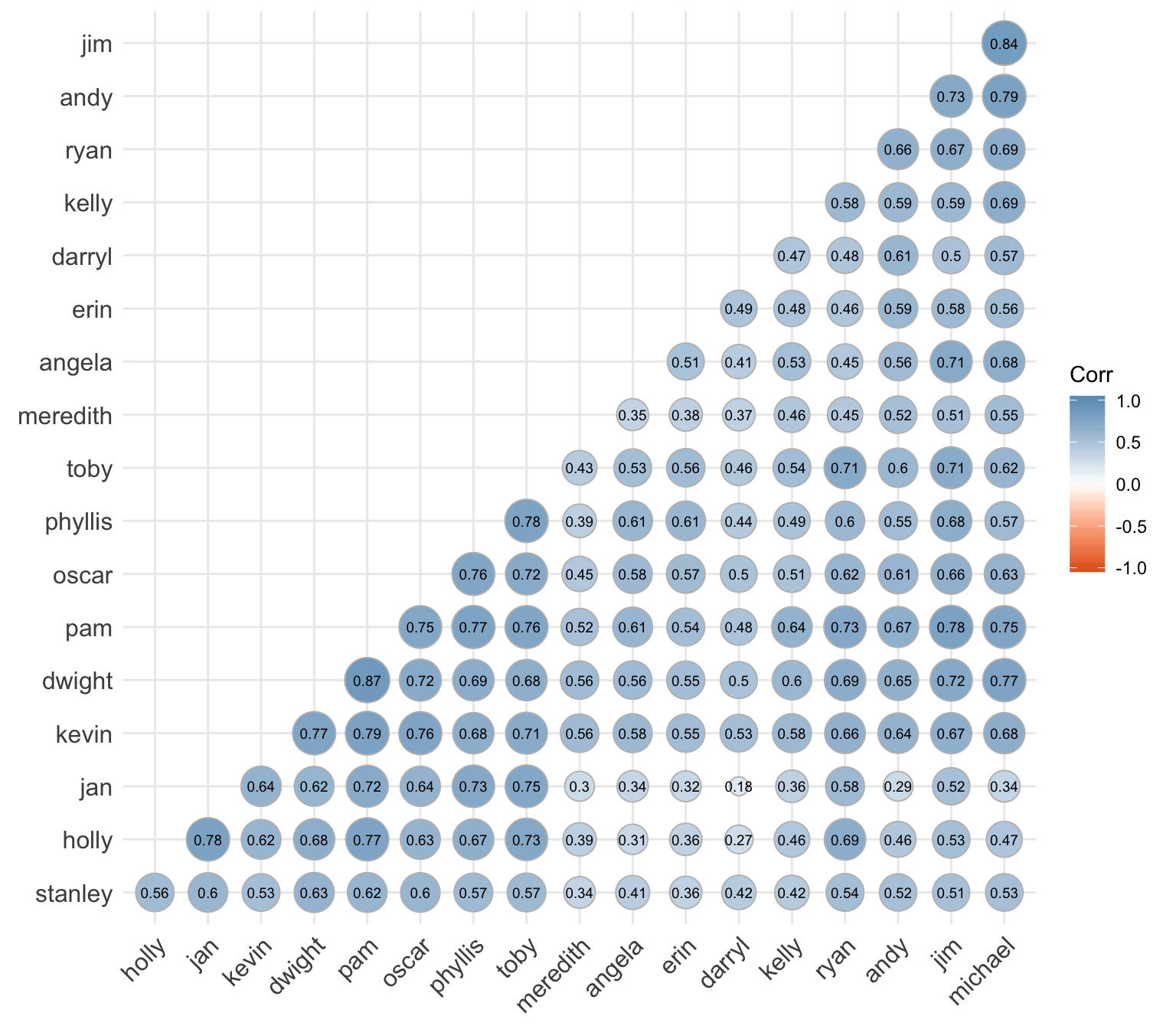
I was a little surprised to find that the two characters who’s words are most correlated are Dwight and Pam. Michael and Jim are a close second.
Jan and Darryl had the least similar vocabularies.
Given this info, I wanted to see which words Dwight and Pam shared.
pam_dwight_words <- frequency_by_character %>%
  select(word, pam, dwight) %>%
  ggplot(aes(x = pam, y = dwight, color = abs(pam - dwight), label = word)) +
  geom_abline(color = "gray40", lty = 2) +
  geom_jitter(alpha = 0.1, size = 2.5, width = 0.3, height = 0.3) +
  scale_x_log10(labels = percent_format()) +
  scale_y_log10(labels = percent_format()) +
  labs(x = "Pam",
       y = "Dwight",
       title = "Word Frequncy Comparison: Dwight and Pam") +
  theme(legend.position = "none")

ggplotly(pam_dwight_words, tooltip = c("word"))
Words in this plot are said at least once by Dwight and Pam. The words closer to the line indicate similar word frequencies between the two characters and those farther from the line are more frequently used by one character vs. the other. You can scroll over the points to see each word. For example, “money”, “school”, and “leave” are used with similar frequencies. However, words like “Schrute”, “regional”, “damn”, and “Mose” are used more frequently by Dwight and words like “Cece”, “mural”, “dating”, and “wedding” are more frequently used by Pam.
Comparing Word Usage
In addition to comparing raw word frequencies, we can determine which words are more or less likely to come from each character using the log odds ratio.
word_ratios_dwight_pam <- tidy_tokens_no_stop %>%
  filter(speaker %in% c("dwight", "pam")) %>%
  count(word, speaker) %>%
  filter(n >= 10) %>%
  spread(speaker, n, fill = 0) %>%
  mutate_if(is.numeric, funs((. + 1) / sum(. + 1))) %>%
  mutate(log_ratio = log2(dwight / pam)) %>%
  arrange(desc(log_ratio))
Which words have about the same likelihood of being said by Dwight and Pam? A log odds ratio near 0 means the two characters had an equal likelihood of saying a given word.
| word | dwight | pam | log_ratio |
|---|---|---|---|
| check | 0.0029204 | 0.0029205 | -0.0000526 |
| desk | 0.0034513 | 0.0034358 | 0.0064903 |
| stanley | 0.0041593 | 0.0041230 | 0.0126425 |
| minutes | 0.0035398 | 0.0036076 | -0.0273732 |
| eat | 0.0026549 | 0.0025769 | 0.0430162 |
| money | 0.0028319 | 0.0029205 | -0.0444467 |
| andy | 0.0066372 | 0.0068717 | -0.0500933 |
| wait | 0.0107080 | 0.0103075 | 0.0549888 |
| walk | 0.0023009 | 0.0024051 | -0.0638991 |
| pam | 0.0098230 | 0.0103075 | -0.0694586 |
Dwight and Pam are both equally likely to say “check”, “desk”, “Stanley”, and “minutes”.
Now let’s look at the words that are most likely to be said by Dwight vs. the words most likely to be said by Pam.
word_ratios_dwight_pam %>%
  group_by(direction = ifelse(log_ratio < 0, 'Pam', "Dwight")) %>%
  top_n(15, abs(log_ratio)) %>%
  ungroup() %>%
  mutate(word = reorder(word, log_ratio)) %>%
  ggplot(aes(word, log_ratio, color = direction)) +
  geom_segment(aes(x = word, xend = word,
                     y = 0, yend = log_ratio),
                 size = 1.1, alpha = 0.6) +
  geom_point(size = 2.5) +
  coord_flip() +
  theme_minimal() +
  labs(x = NULL,
       y = "Relative Occurrence",
       title = "Words Paired with Dwight and Pam") +
  theme(plot.title = element_text(hjust = 0.5),
        legend.title = element_blank()) +
  scale_y_continuous(breaks = seq(-6, 6),
                     labels = c("64x", "32x", "16x","8x", "4x", "2x",
                                  "Same", "2x", "4x", "8x", "16x", "32x", "64x")) +
  scale_color_manual(values = c("#daad62", "#9c311f"))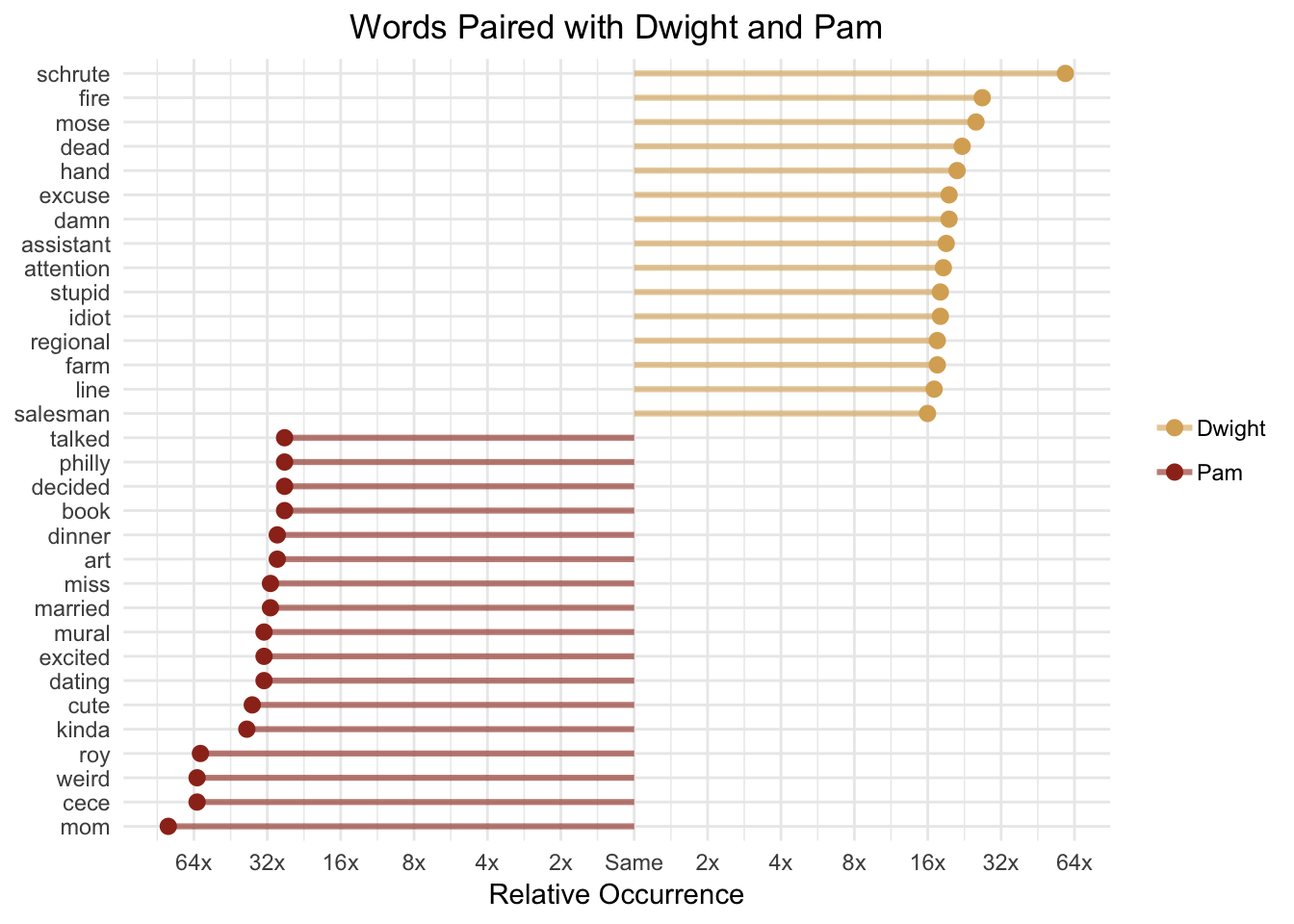
Dwight is more than sixteen times as likely to talk about “Schrute” (his last name and the name of his farm, Schrute Farms), “fire”, “Mose” (his cousin), and “death” whereas Pam is more likely to talk about her “mom”, “Cece” (her kid), and “Roy” (her former fiance). It’s important to note that we’re working with a relatively small dataset, which partially explains why some of the log ratios are so large.

Word Relationships
In addition to analyzing individual words, we can also tokenize the data by n-grams. N-grams are consecutive sequences of words, where n is the number of words in the sequence. For example, if we wanted to look at two word sequences (bigrams), we can use the unnest_tokens() function to do so.
tidy_bigrams <- mod_data %>%
  select(line = id, line_text_mod, everything(), -line_text, -actions, -deleted) %>%
unnest_tokens(bigram, line_text_mod, token = "ngrams", n = 2)| line | season | episode | scene | speaker | bigram |
|---|---|---|---|---|---|
| 1 | 1 | 1 | 1 | michael | all right |
| 1 | 1 | 1 | 1 | michael | right jim |
| 1 | 1 | 1 | 1 | michael | jim your |
| 1 | 1 | 1 | 1 | michael | your quarterlies |
| 1 | 1 | 1 | 1 | michael | quarterlies look |
| 1 | 1 | 1 | 1 | michael | look very |
| 1 | 1 | 1 | 1 | michael | very good |
| 1 | 1 | 1 | 1 | michael | good how |
| 1 | 1 | 1 | 1 | michael | how are |
| 1 | 1 | 1 | 1 | michael | are things |
Just like with individual words, we can remove stop words from bigrams and calculate tf-idf to give us bigrams that are unique to individual characters.
# remove stop words from bigrams and calculate tf-idf
bigram_tf_idf_no_stop <- tidy_bigrams %>%
  filter(speaker %in% main_characters, !is.na(bigram)) %>%
  separate(bigram, c("word1", "word2"), sep = " ") %>%
  filter(!word1 %in% custom_stop_words$word,
         !word2 %in% custom_stop_words$word) %>%
  unite(bigram, word1, word2, sep = " ") %>%
  count(speaker, bigram) %>%
  bind_tf_idf(bigram, speaker, n) %>%
  arrange(desc(tf_idf))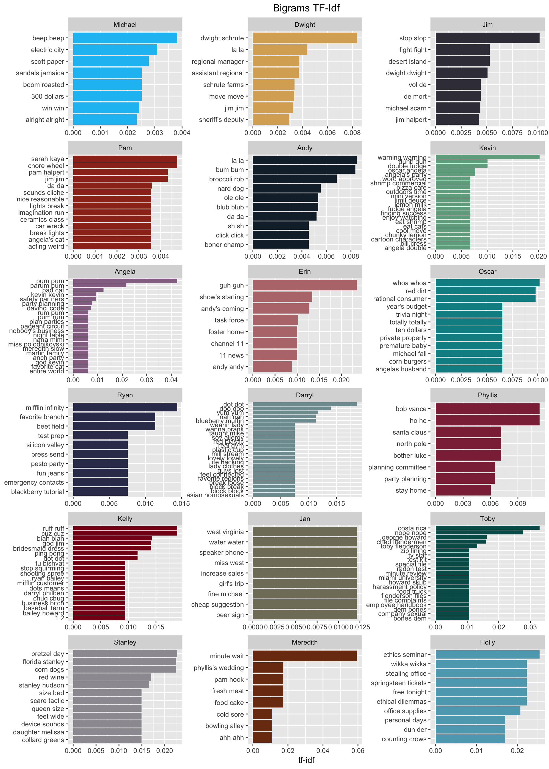

If we wanted to understand the relationships between words that co-occur, but aren’t necessarily right next to each other in a sentence, we can use the widyr package. The pairwise_cor() function gives us a measure of how frequently two words appear together relative to how frequently they appear separately. Here we’ll explore the words “corporate”, “Scranton”, “office”, and “love” by scene to discover which words are most correlated to them.
word_cors_scene <- tidy_tokens_no_stop %>%
  unite(se_ep_sc, season, episode, scene) %>%
  group_by(word) %>%
  filter(n() >= 20) %>%
  pairwise_cor(word, se_ep_sc, sort = TRUE)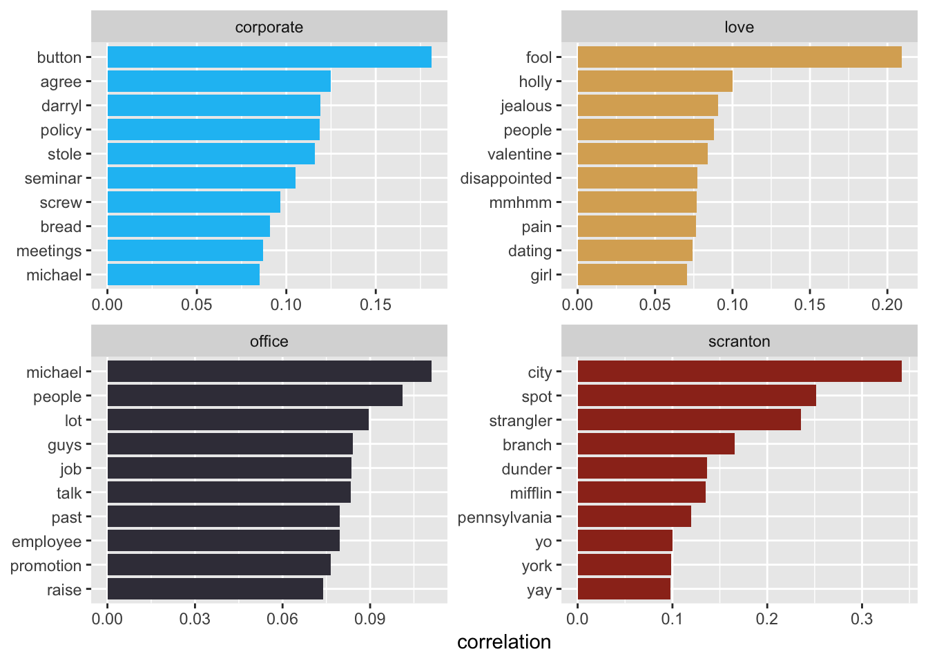
We can also use a network graph to visualize word correlations over a certain threshold.
set.seed(1234)

word_cors_scene %>%
  filter(correlation > .30) %>%
  graph_from_data_frame() %>%
  ggraph(layout = "fr") +
  geom_edge_link(aes(edge_alpha = correlation), show.legend = FALSE) +
  geom_node_point(color = "lightblue", size = 5) +
  geom_node_text(aes(label = name), repel = TRUE) +
  theme_void()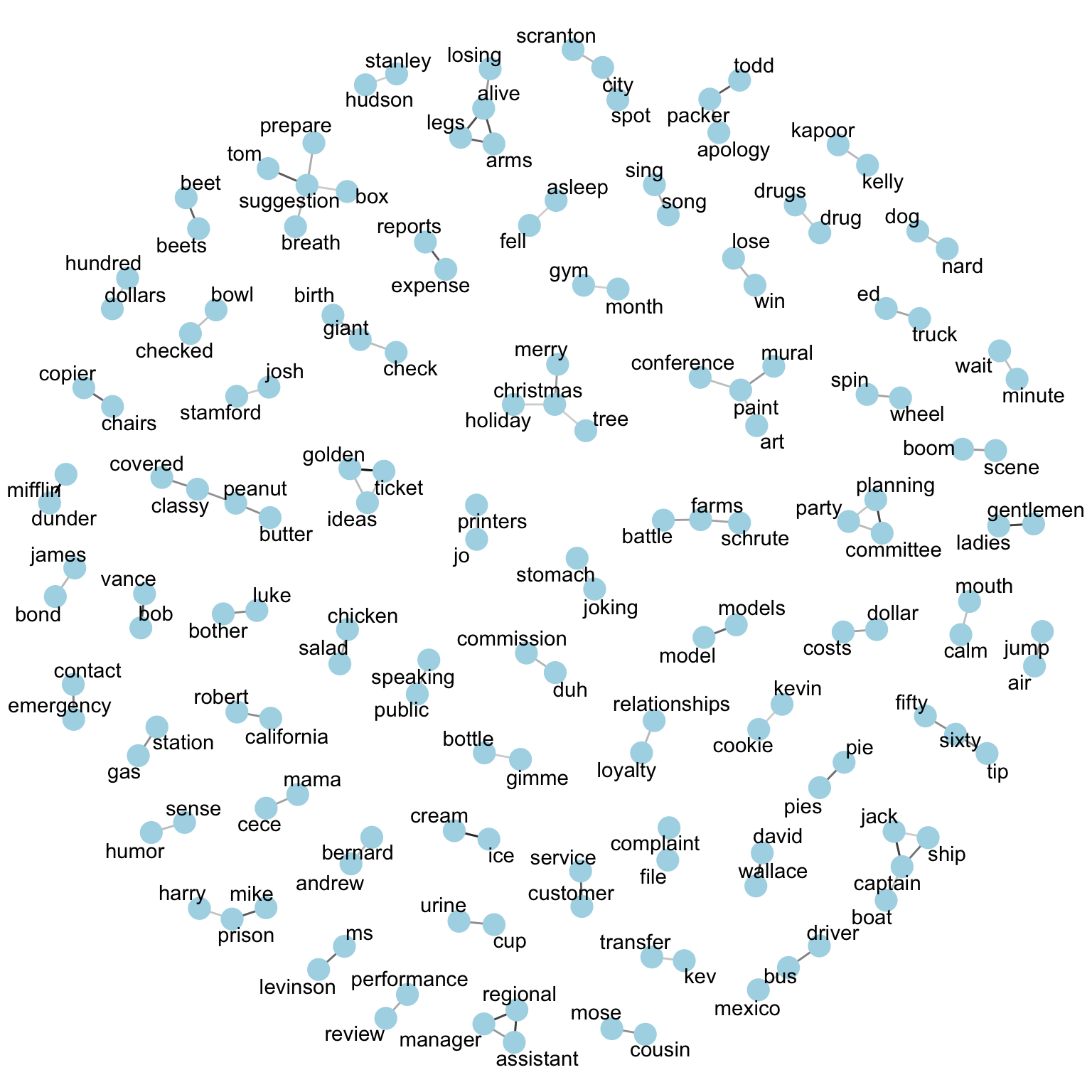
Parts of Speech Tagging
Another way to better understand word relationships is to use the cleanNLP package for parts of speech tagging. Essentially this package analyzes the text and determines which words are nouns, verbs, adjectives, etc. and it gives word dependencies. It can also perform named entity recognition which identifies entities that can be defined by proper names and categorizes them as people, locations, events, organizations, etc. The cleanNLP offers a few different back ends to perform the text annotation. I’m going to use the spaCy back end, which requires the reticulate package and python.
tif_data <- mod_data %>%
  select(id, line_text_mod, season, episode, scene, speaker)

cnlp_init_spacy()
obj <- cnlp_annotate(tif_data, as_strings = TRUE)names(obj)## [1] "coreference" "dependency" "document" "entity" "sentence"
## [6] "token" "vector"The resulting annotation object is a list of data frames (and one matrix), similar to a set of tables within a database.
First let’s look at the entities table.
entities <- cnlp_get_entity(obj)| id | sid | tid | tid_end | entity_type | entity |
|---|---|---|---|---|---|
| 1 | 1 | 3 | 3 | PERSON | Jim |
| 6 | 3 | 3 | 4 | PERSON | Michael Scott |
| 6 | 4 | 7 | 10 | ORG | Dunder Mifflin Paper Products |
| 7 | 1 | 10 | 11 | PRODUCT | Dunder Mifflin |
| 7 | 1 | 13 | 14 | DATE | 12 years |
| 7 | 1 | 18 | 18 | CARDINAL | four |
| 7 | 7 | 2 | 2 | ORG | Beesly |
| 7 | 10 | 2 | 2 | PERSON | Pam |
| 9 | 1 | 13 | 18 | DATE | her a couple of years ago |
| 16 | 6 | 5 | 6 | PERSON | Spencer Gifts |
Here we see the entity identified and the entity type. The entity types identified here are pretty good, but there are some mistakes, which require review and clean up. We can join this table back to the original data by id to bring in the metadata such as speaker. From there we can again use tf-idf to see which entities were uniquely talked about by a given character.
meta <- mod_data %>%
  select(1:4, 6)

tf_idf_entities <- entities %>%
  mutate_at(vars(id), as.integer) %>%
  left_join(meta, by = "id") %>%
  filter(speaker %in% main_characters) %>%
  count(entity, speaker, sort = TRUE) %>%
  bind_tf_idf(entity, speaker, n)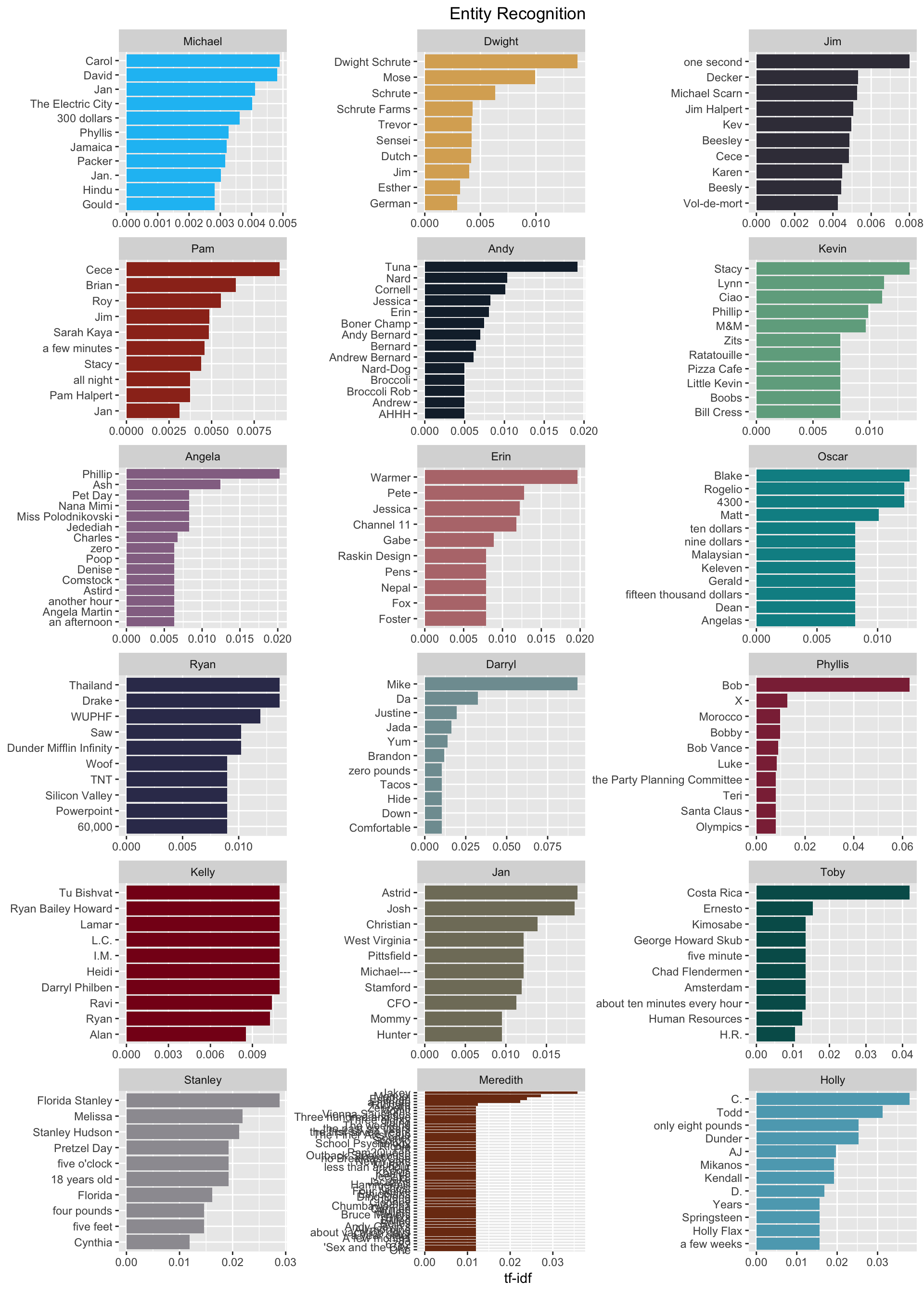
The annotation object also has table called dependencies.
dependencies <- cnlp_get_dependency(obj, get_token = TRUE)| id | sid | tid | tid_target | relation | relation_full | word | lemma | word_target | lemma_target |
|---|---|---|---|---|---|---|---|---|---|
| 1 | 1 | 3 | 1 | det | NA | Jim | jim | All | all |
| 1 | 1 | 3 | 2 | amod | NA | Jim | jim | right | right |
| 1 | 1 | 0 | 3 | ROOT | NA | ROOT | ROOT | Jim | jim |
| 1 | 1 | 3 | 4 | punct | NA | Jim | jim | . | . |
| 1 | 2 | 2 | 1 | poss | NA | quarterlies | quarterly | Your | -PRON- |
| 1 | 2 | 3 | 2 | nsubj | NA | look | look | quarterlies | quarterly |
| 1 | 2 | 0 | 3 | ROOT | NA | ROOT | ROOT | look | look |
| 1 | 2 | 5 | 4 | advmod | NA | good | good | very | very |
| 1 | 2 | 3 | 5 | acomp | NA | look | look | good | good |
| 1 | 2 | 3 | 6 | punct | NA | look | look | . | . |
This provides a lot of really useful information! We can see each word, lemma, word target, and lemma target. According to Wikipedia “a lemma (plural lemmas or lemmata) is the canonical form, dictionary form, or citation form of a set of words. For example, run, runs, ran and running are forms of the same lexeme, with run as the lemma.” This table provides the grammatical relationship between the word/lemma and the word_target/lemma_target. From this we can get common verb noun phrases, for example, by filtering for the direct object relationship.
dobj <- dependencies %>%
  filter(relation == "dobj") %>%
  select(id = id, verb = lemma, noun = word_target) %>%
  select(id, verb, noun) %>%
  count(verb = tolower(verb), noun = tolower(noun), sort = TRUE)
What is a direct object, you ask?

The direct object of a verb is the thing being acted upon (i.e., the receiver of the action). From our earlier analysis, we saw that characters commonly used the words “god”, “time”, “love”, and “office”. Let’s try to put a little more context around these words and see how they are used when they are direct objects.
dobj_packed_bubble <- function(data, word) {

  filtered <- data %>%
    filter(noun == word)

  packing <- circleProgressiveLayout(filtered$n, sizetype = "area")

  verts <- circleLayoutVertices(packing, npoints = 50)

  combined <- filtered %>%
    bind_cols(packing)

  plot <- ggplot(data = verts) +
  geom_polygon(aes(x, y, group = id, fill = factor(id)), color = "black", show.legend = FALSE, alpha = 0.8) +
  coord_equal() +
  geom_text(data = combined, aes(x, y, label = ifelse(radius > .9, verb, "")), check_overlap = TRUE) +
  theme_minimal() +
  labs(title = str_to_title(word)) +
  theme(plot.title = element_text(hjust = 0.5),
        axis.title = element_blank(),
        axis.ticks = element_blank(),
        axis.text = element_blank())
}

direct_objects <- c("god", "time", "love", "office")
plots <- setNames(map(direct_objects, ~ dobj_packed_bubble(dobj, .)), direct_objects)

plots[["god"]] + plots[["time"]] + plots[["love"]] + plots[["office"]] + plot_layout(ncol = 2)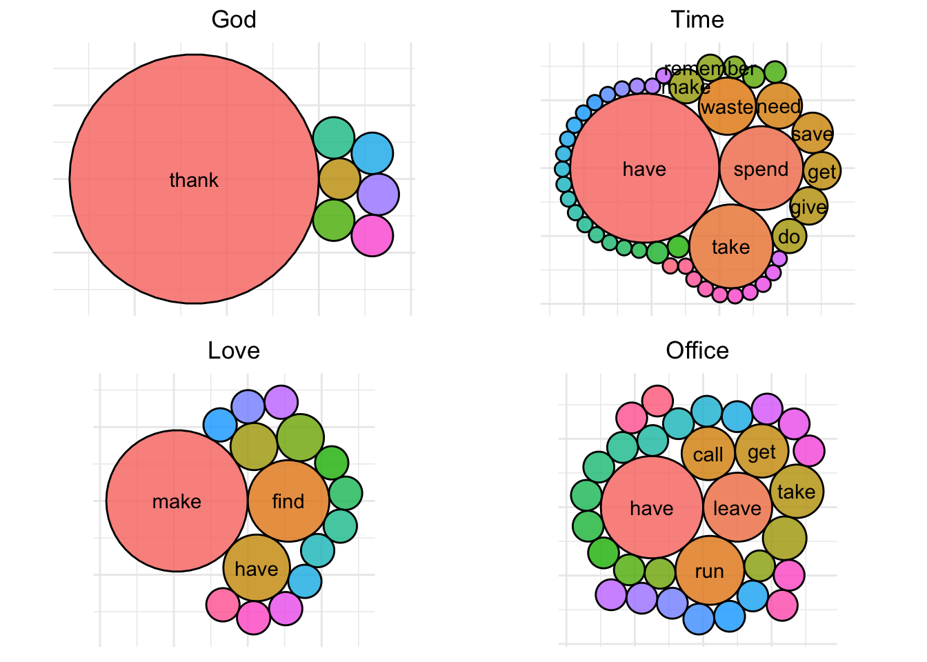
We can see that when “god” is the direct object, someone is usually thanking god. For “love”, the office characters are generally talking about making, having, and finding love, so on and so forth.
This post is getting pretty long, but if you’ve stuck with me this far, I’ll just leave this here…
| line |
|---|
| i’m good. |
| uh… my mother’s coming. |
| that is really hard. |
| you really think you can go all day long? |
| well, you always left me satisfied and smiling, so… |
| why did you get it so big? |
| does the skin look red and swollen? |
| you already did me. |
| even if it didn’t, at least we put this matter to bed. |
| they taste so good in my mouth. |
| i want you to think about it long and hard. |
| let’s just blow this party off. |
| why is this so hard? |
| i need two men on this. |
| dip it in the water so it will slide down your gullet more easily. |
| can you make that straighter? |
| and up comes the toolbar. |
| that’s what i said. |
| when things sort of get hard. |
| and you were directly under her the entire time? |
| excuse me? |
| come again? |
| and you’re hardly my first! |
| force it in as deep as you can. |
| it was easy to get in but impossible to rise up. |
| yeah, well, if you’re only free till three on sunday and i can’t get there till one, then it’s gonna be pretty tight. |
| it squeaks when you bang it. |
| don’t make it harder than it has to be. |
| dwight, get out of my nook! |
| this is huge. |
| so instead, you screwed me? |
| you need to get back on top. |
| you are making this harder than it has to be. |
| no, comedy is a place where the mind goes to tickle itself. |
| i’m not saying it won’t be hard. but we can make it work. |
| this is gonna feel so good, getting this thing off my chest. |
| ’cause there’s just no way you guys are making this magic with just your mouths. |
| i can’t believe you came. |