This was a project that I originally did for my Data Warehousing class in grad school using Microsoft SQL server and SSIS. I’ve been taking a lot of datacamp courses lately and wanted to put what I learned about the tidyverse into action. This project has a lot of data manipulation and cleanup tasks, so I thought it would be a good candidate to convert what I did in grad school to R and MySQL. Enjoy!
Abstract
Using a dimensional model, data warehouse, and Tableau I explored data from the College Scorecard and NCAA Division I FBS football games to create a data-driven approach to school selection for college football fans.
Data Warehouse Opportunity and Objectives
For many students in the United States, NCAA Division I football is an important part of their student life and college experience. It is also my biased opinion that college football is fun to watch, especially when you have an emotional investment in one of the teams playing. Thus, I saw an opportunity to create a data-driven approach to school selection for college football fans.
The data-driven approach included several objectives:
- Retrieve data from the College Scorecard using the available API
- Scrape NCAA Division I FBS college football game scores from the web
- Cleanup and transform the data
- Create a dimensional data model
- Load the data into a MySQL data warehouse running on AWS
- Create an interactive dashboard that allows users to input certain criteria regarding school location, size, graduation rate, total cost, etc. and get back a filtered list of schools showing a map of the school location, tuition and fee cost per win, point differential per game, points per game, etc.
library(RMySQL)
library(data.table)
library(utils)
library(tidyverse)
library(rscorecard)
library(rvest)
library(stringdist)
library(lubridate)
Source Data
College Scorecard School Data
I am using the available API provided by College Scorecard to extract the relevant school data. The College Scorecard combines data from the Integrated Postsecondary Education Data System (IPEDS), National Student Loan Data System (NSLDS), and various other sources into one dataset and makes it available through an API. The extraction process includes selecting the desired data fields (there are a ton to choose from), determining which years to pull data for, and creating the API call to return the data. The latest full dataset available is for the 2015-2016 school year. I will be extracting the last 5 school years worth of data (2011-2012, 2012-2013, 2013-2014, 2014-2015, 2015-2016).
In R, there is an existing package called rscorecard that “is simply a method for converting idiomatic R code into a properly formatted URL string that is then queried.” This package does require an API key which I requested here. I added the API key to a .Renviron file to maintain security best practices.
years <- seq(2011, 2015)# get school data for all 4-year schools that are public or private non-profit for desired years and combine it all into one tibble
school_data_staging <- map_dfr(years, ~
sc_init() %>%
sc_filter(ICLEVEL == 1, CONTROL == 1:2) %>%
sc_select(UNITID, OPEID, OPEID6, INSTNM, CITY, STABBR, ZIP, INSTURL, MAIN, CONTROL, REGION, LATITUDE, LONGITUDE, ADM_RATE, SATVR25, SATVR75, SATMT25, SATMT75, SATVRMID, SATMTMID, ACTCM25, ACTCM75, ACTEN25, ACTEN75, ACTMT25, ACTMT75, ACTCMMID, ACTENMID, ACTMTMID, UGDS, TUITIONFEE_IN, TUITIONFEE_OUT, C150_4, RET_FT4, PCTFLOAN, GRAD_DEBT_MDN, GRAD_DEBT_MDN10YR, LOAN_EVER, ALIAS, C100_4, ICLEVEL) %>%
sc_year(.x) %>%
sc_get()
)| satvrmid | c100_4 | loan_ever | satmt75 | actcm75 | acten75 | actmtmid | main | city | satvr25 | pctfloan | ret_ft4 | iclevel | zip | latitude | satmtmid | satmt25 | ugds | actcmmid | stabbr | alias | unitid | region | longitude | instnm | actcm25 | c150_4 | tuitionfee_in | control | grad_debt_mdn | actmt75 | opeid6 | tuitionfee_out | insturl | acten25 | actenmid | satvr75 | opeid | actmt25 | adm_rate | grad_debt_mdn10yr | year |
|---|---|---|---|---|---|---|---|---|---|---|---|---|---|---|---|---|---|---|---|---|---|---|---|---|---|---|---|---|---|---|---|---|---|---|---|---|---|---|---|---|---|
| 570 | 0.2488538 | 0.8158580 | 630 | 27 | 28 | 25 | 1 | Tampa | 520 | 0.4489 | 0.8752 | 1 | 33620-9951 | 28.05665 | 585 | 540 | 29232 | 25 | FL | USF Main Campus |USF Tampa Campus |USF Tampa |USF | 137351 | 5 | -82.41588 | University of South Florida-Main Campus | 23 | 0.5171 | 5800 | 1 | 17500 | 27 | 1537 | 14990 | www.usf.edu | 22 | 25 | 620 | 153700 | 23 | 0.3805 | NA | 2011 |
| NA | NA | 0.6935032 | NA | NA | NA | NA | 1 | Clearwater | NA | 0.3461 | NA | 1 | 33760-2822 | 27.90260 | NA | NA | 28077 | NA | FL | SPC, Saint Petersburg College, St. Petersburg College | 137078 | 5 | -82.71732 | St Petersburg College | NA | 0.2766 | 2988 | 1 | 12500 | NA | 1528 | 10897 | www.spcollege.edu | NA | NA | NA | 152800 | NA | NA | NA | 2011 |
| NA | NA | 0.2994798 | NA | NA | NA | NA | 1 | Fort Lauderdale | NA | 0.1406 | NA | 1 | 33301 | 26.07972 | NA | NA | 37774 | NA | FL | BC | 132709 | 5 | -80.23541 | Broward College | NA | 0.2536 | 2446 | 1 | 6500 | NA | 1500 | 2446 | www.broward.edu | NA | NA | NA | 150000 | NA | NA | NA | 2011 |
| NA | 0.1111111 | 0.7887324 | NA | NA | NA | NA | 1 | Lithonia | NA | 0.5049 | 0.0000 | 1 | 30038-9869 | 33.69798 | NA | NA | 482 | NA | GA | NA | 135364 | 5 | -84.12365 | Luther Rice College & Seminary | NA | 0.1111 | 5520 | 2 | 18750 | NA | 31009 | 5520 | www.lutherrice.edu | NA | NA | NA | 3100900 | NA | NA | NA | 2011 |
| NA | NA | 0.5679661 | NA | NA | NA | NA | 1 | Bradenton | NA | 0.2949 | NA | 1 | 34207 | 27.43607 | NA | NA | 10182 | NA | FL | SCF | 135391 | 5 | -82.59174 | State College of Florida-Manatee-Sarasota | NA | 0.3210 | 3074 | 1 | 9450 | NA | 1504 | 11597 | www.scf.edu | NA | NA | NA | 150400 | NA | NA | NA | 2011 |
Football Data
For the football data, I am going to scrape data from http://www.sports-reference.com, a sports statistics clearinghouse that allows free downloads of data. You can export this data to CSVs, but I’m going to scrape it so I don’t have to deal with multiple CSV files. To mirror the school data, I will be extracting the data for the same school years as mentioned above (2011-2012, 2012-2013, 2013-2014, 2014-2015, 2015-2016). I’ll also be getting data for bowl games. The bowl data is on a separate webpage of the site.
get_football_data <- function(games, years) {
  if (!(games %in% c("schedule", "bowls"))) {
    stop("Game arg must be either 'schedule' or 'bowls'", call. = FALSE)
  }
  # create urls based on the desired years and if user wants all games or bowl games
  urls <- paste0("https://www.sports-reference.com/cfb/years/",years,"-",games,".html")

  # get html from urls
  urls_html <- map(urls, ~ read_html(.x))

  # get the data for each url and combine it into one data table
  football_data <- rbindlist(map(urls_html, ~ .x %>%
                                   html_nodes("table") %>%
                                   .[[1]] %>%
                                   html_table()), fill = TRUE) # fill = true here because different years have different columns included in the data
  return(football_data)
}
football_data_staging <- get_football_data("schedule", years)
football_data_staging_bowls <- get_football_data("bowls", years)| Rk | Wk | Date | Day | Winner | Pts | V1 | Loser | Pts | Notes | Time | TV |
|---|---|---|---|---|---|---|---|---|---|---|---|
| 1 | 1 | Sep 1, 2011 | Thu | Arizona State | 48 | California-Davis | 14 | NA | NA | ||
| 2 | 1 | Sep 1, 2011 | Thu | Bowling Green State | 32 | @ | Idaho | 15 | NA | NA | |
| 3 | 1 | Sep 1, 2011 | Thu | Central Michigan | 21 | South Carolina State | 6 | NA | NA | ||
| 4 | 1 | Sep 1, 2011 | Thu | Florida International | 41 | North Texas | 16 | NA | NA | ||
| 5 | 1 | Sep 1, 2011 | Thu | Georgia Tech | 63 | Western Carolina | 21 | NA | NA |
| Date | Bowl | Winner | Pts | Loser | Pts | Notes | Gametime | TV |
|---|---|---|---|---|---|---|---|---|
| 2012-01-09 | BCS Championship | Alabama | 21 | Louisiana State | 0 | New Orleans, LA | NA | NA |
| 2012-01-08 | GoDaddy.com Bowl | Northern Illinois | 38 | Arkansas State | 20 | Mobile, AL | NA | NA |
| 2012-01-07 | BBVA Compass Bowl | Southern Methodist | 28 | Pittsburgh | 6 | Birmingham, AL | NA | NA |
| 2012-01-06 | Cotton Bowl | Arkansas | 29 | Kansas State | 16 | Arlington, TX | NA | NA |
| 2012-01-04 | Orange Bowl | West Virginia | 70 | Clemson | 33 | Miami, FL | NA | NA |
Data Cleanup
Now that I have all of the school and football data, I need to clean it up.
School Data
I’ll start with the school data. Overall, it’s in pretty good shape. The main things to do are rename the columns so they are a little more user friendly and decode columns like “CONTROL”, “ICLEVEL”, “REGION”, etc. so that instead of containing numbers they contain what those numbers mean (e.g. a “CONTROL” value of 1 means it is a public school).
I’ll also include the full state name based on the state abbreviation. The decoded values can be found in the College Scorecard data dictionary.
clean_school_data <- function(dirty_data) {
  state_lookups <- read_csv("https://raw.githubusercontent.com/jennaallen/football_schools/master/lookups.csv") %>%
    filter(VariableName == "State abbreviation (HD2016)") %>%
    select(Value, ValueLabel)

  clean_data <- dirty_data %>%
    mutate(region = recode(region,
                           "0"  = "US Service schools",
                           "1"  = "New England",
                           "2"  = "Mid East",
                           "3"  = "Great Lakes",
                           "4"  = "Plains",
                           "5"  = "Southeast",
                           "6"  = "Southwest",
                           "7"  = "Rocky Mountains",
                           "8"  = "Far West",
                           "9"  = "Outlying"),
           control = recode(control,
                            "1" = "Public",
                            "2" = "Private not-for-profit"),
           iclevel = recode(iclevel,
                            "1" = "4-year",
                            "2" = "2-year",
                            "3" = "Less-than-2-year"),
           zip = str_sub(zip, end = 5), # keep only the first 5 numbers for zip code; some values are missing dash between zip and zip +4 code
          school_size_category = case_when(ugds < 1000 ~ "Under 1,000",
                                           between(ugds, 1000, 4999) ~ "1,000 - 4,999",
                                           between(ugds, 5000, 9999) ~ "5,000 - 9,999",
                                           between(ugds, 10000, 19999) ~ "10,000 - 19,999",
                                           ugds > 20000 ~ "20,000 and above",
                                           TRUE ~ NA_character_)) %>%
    left_join(state_lookups, by = c("stabbr" = "Value")) %>%
    rename("ACT_composite_25th_percentile" = actcm25,
           "ACT_composite_75th_percentile" = actcm75,
           "ACT_composite_midpoint" = actcmmid,
           "ACT_english_25th_percentile" = acten25,
           "ACT_english_75th_percentile" = acten75,
           "ACT_english_midpoint" = actenmid,
           "ACT_math_25th_percentile" = actmt25,
           "ACT_math_75th_percentile" = actmt75,
           "ACT_math_midpoint" = actmtmid,
           "school_admission_rate" = adm_rate,
           "school_alias" = alias,
           "school_graduation_rate_4yrs" = c100_4,
           "school_graduation_rate_6yrs" = c150_4,
           "school_city" = city,
           "school_control" = control,
           "school_median_debt_graduates" = grad_debt_mdn,
           "school_median_debt_graduates_monthly_payments" = grad_debt_mdn10yr,
           "school_name" = instnm,
           "school_url" = insturl,
           "school_latitude" = latitude,
           "school_level" = iclevel,
           "school_students_with_any_loan" = loan_ever,
           "school_longitude" = longitude,
           "school_main_campus_flag" = main,
           "school_opeid8" = opeid,
           "school_opeid6" = opeid6,
           "school_federal_loan_rate" = pctfloan,
           "school_region" = region,
           "school_retention_rate" = ret_ft4,
           "SAT_math_25th_percentile" = satmt25,
           "SAT_math_75th_percentile" = satmt75,
           "SAT_math_midpoint" = satmtmid,
           "SAT_reading_25th_percentile" = satvr25,
           "SAT_reading_75th_percentile" = satvr75,
           "SAT_reading_midpoint" = satvrmid,
           "school_st_abbr" = stabbr,
           "school_in_state_price" =  tuitionfee_in,
           "school_out_state_price" = tuitionfee_out,
           "school_size" = ugds,
           "school_id" = unitid,
           "school_state" = ValueLabel,
           "school_year_start" =  year,
           "school_zip" = zip)
  return(clean_data)
}
school_data_transform <- clean_school_data(school_data_staging)| SAT_reading_midpoint | school_graduation_rate_4yrs | school_students_with_any_loan | SAT_math_75th_percentile | ACT_composite_75th_percentile | ACT_english_75th_percentile | ACT_math_midpoint | school_main_campus_flag | school_city | SAT_reading_25th_percentile | school_federal_loan_rate | school_retention_rate | school_level | school_zip | school_latitude | SAT_math_midpoint | SAT_math_25th_percentile | school_size | ACT_composite_midpoint | school_st_abbr | school_alias | school_id | school_region | school_longitude | school_name | ACT_composite_25th_percentile | school_graduation_rate_6yrs | school_in_state_price | school_control | school_median_debt_graduates | ACT_math_75th_percentile | school_opeid6 | school_out_state_price | school_url | ACT_english_25th_percentile | ACT_english_midpoint | SAT_reading_75th_percentile | school_opeid8 | ACT_math_25th_percentile | school_admission_rate | school_median_debt_graduates_monthly_payments | school_year_start | school_size_category | school_state |
|---|---|---|---|---|---|---|---|---|---|---|---|---|---|---|---|---|---|---|---|---|---|---|---|---|---|---|---|---|---|---|---|---|---|---|---|---|---|---|---|---|---|---|---|
| 570 | 0.2488538 | 0.8158580 | 630 | 27 | 28 | 25 | 1 | Tampa | 520 | 0.4489 | 0.8752 | 4-year | 33620 | 28.05665 | 585 | 540 | 29232 | 25 | FL | USF Main Campus |USF Tampa Campus |USF Tampa |USF | 137351 | Southeast | -82.41588 | University of South Florida-Main Campus | 23 | 0.5171 | 5800 | Public | 17500 | 27 | 1537 | 14990 | www.usf.edu | 22 | 25 | 620 | 153700 | 23 | 0.3805 | NA | 2011 | 20,000 and above | Florida |
| NA | NA | 0.6935032 | NA | NA | NA | NA | 1 | Clearwater | NA | 0.3461 | NA | 4-year | 33760 | 27.90260 | NA | NA | 28077 | NA | FL | SPC, Saint Petersburg College, St. Petersburg College | 137078 | Southeast | -82.71732 | St Petersburg College | NA | 0.2766 | 2988 | Public | 12500 | NA | 1528 | 10897 | www.spcollege.edu | NA | NA | NA | 152800 | NA | NA | NA | 2011 | 20,000 and above | Florida |
| NA | NA | 0.2994798 | NA | NA | NA | NA | 1 | Fort Lauderdale | NA | 0.1406 | NA | 4-year | 33301 | 26.07972 | NA | NA | 37774 | NA | FL | BC | 132709 | Southeast | -80.23541 | Broward College | NA | 0.2536 | 2446 | Public | 6500 | NA | 1500 | 2446 | www.broward.edu | NA | NA | NA | 150000 | NA | NA | NA | 2011 | 20,000 and above | Florida |
| NA | 0.1111111 | 0.7887324 | NA | NA | NA | NA | 1 | Lithonia | NA | 0.5049 | 0.0000 | 4-year | 30038 | 33.69798 | NA | NA | 482 | NA | GA | NA | 135364 | Southeast | -84.12365 | Luther Rice College & Seminary | NA | 0.1111 | 5520 | Private not-for-profit | 18750 | NA | 31009 | 5520 | www.lutherrice.edu | NA | NA | NA | 3100900 | NA | NA | NA | 2011 | Under 1,000 | Georgia |
| NA | NA | 0.5679661 | NA | NA | NA | NA | 1 | Bradenton | NA | 0.2949 | NA | 4-year | 34207 | 27.43607 | NA | NA | 10182 | NA | FL | SCF | 135391 | Southeast | -82.59174 | State College of Florida-Manatee-Sarasota | NA | 0.3210 | 3074 | Public | 9450 | NA | 1504 | 11597 | www.scf.edu | NA | NA | NA | 150400 | NA | NA | NA | 2011 | 10,000 - 19,999 | Florida |
Football Data
The football data is a bit more messy than the school data. For example, the row headers are sometimes repeated in the middle of the dataset. Also, for some schools the ranking precedes the school name (i.e. “(2) Alabama”). As a part of the cleaning process for the football data, I’m also going to join in the bowl game information and create flags for which games were bowl games and which ones were national championship games.
clean_football_data <- function(all_games, bowls) {
  clean_bowls <- bowls %>%
    set_tidy_names() %>%
    as_tibble() %>%
    mutate_at(vars(Date), ymd) %>%
    select(Date, Bowl, Winner)
  clean_all_games <- all_games %>%
    set_tidy_names() %>%
    as_tibble() %>%
    rename(school_points = Pts..6, opponent_points = Pts..9, home_away = V1) %>%
    mutate_all(funs(replace(., . == '', NA))) %>%
    filter(!(Rk %in% "Rk") & !(Notes %like% "Cancelled")) %>%
    mutate(school_rank = str_extract(Winner, "\\d{1,2}"),
           opponent_rank = str_extract(Loser, "\\d{1,2}"),
           school = str_replace(Winner, "\\(\\d{1,2}\\)\\s", ""),
           opponent = str_replace(Loser, "\\(\\d{1,2}\\)\\s", ""),
           school_game_site = case_when(home_away %in% "@" ~ "away",
                                        is.na(Notes) ~ "home",
                                        TRUE ~ "neutral"),
           opponent_game_site = case_when(school_game_site %in% "away" ~ "home",
                                          school_game_site %in% "home" ~ "away",
                                          TRUE ~ "neutral"),
           school_win = as.integer(1),
           opponent_win = as.integer(0)) %>%
    mutate_at(vars(Rk, Wk, school_points, opponent_points, school_rank, opponent_rank), as.integer) %>%
    mutate_at(vars(Date), mdy) %>%
    left_join(clean_bowls, by = c("Date" = "Date", "school" = "Winner")) %>%
    mutate(bowl_flag = if_else(!is.na(Bowl), 1, 0),
           national_championship_flag = if_else(Bowl %like% "Championship", 1, 0)) %>%
    mutate_at(vars(bowl_flag, national_championship_flag), as.integer) %>%
    rename("game_number" = Rk,
           "football_week" = Wk,
           "game_date" = Date,
           "game_day" = Day,
           "football_notes" = Notes,
           "game_time" = Time,
           "game_tv" = TV,
           "bowl" = Bowl) %>%
    select(-Winner, -Loser, -home_away)
  return(clean_all_games)
}
football_data_transform <- clean_football_data(football_data_staging, football_data_staging_bowls)| game_number | football_week | game_date | game_day | school_points | opponent_points | football_notes | game_time | game_tv | school_rank | opponent_rank | school | opponent | school_game_site | opponent_game_site | school_win | opponent_win | bowl | bowl_flag | national_championship_flag |
|---|---|---|---|---|---|---|---|---|---|---|---|---|---|---|---|---|---|---|---|
| 1 | 1 | 2011-09-01 | Thu | 48 | 14 | NA | NA | NA | NA | NA | Arizona State | California-Davis | home | away | 1 | 0 | NA | 0 | 0 |
| 2 | 1 | 2011-09-01 | Thu | 32 | 15 | NA | NA | NA | NA | NA | Bowling Green State | Idaho | away | home | 1 | 0 | NA | 0 | 0 |
| 3 | 1 | 2011-09-01 | Thu | 21 | 6 | NA | NA | NA | NA | NA | Central Michigan | South Carolina State | home | away | 1 | 0 | NA | 0 | 0 |
| 4 | 1 | 2011-09-01 | Thu | 41 | 16 | NA | NA | NA | NA | NA | Florida International | North Texas | home | away | 1 | 0 | NA | 0 | 0 |
| 5 | 1 | 2011-09-01 | Thu | 63 | 21 | NA | NA | NA | NA | NA | Georgia Tech | Western Carolina | home | away | 1 | 0 | NA | 0 | 0 |
Now that the school and football data are clean, I’m ready to create the data model.
Dimensional Model
I am going to store this data in MySQL running on AWS RDS. To initially setup an AWS RDS instance, I loosely followed these directions.
For this project, I’m going to use a star schema. The first step in creating the dimensional data model is profiling the data in order to better understand how the data from the two different sources fits together. During this profiling step, I determined what data types best fit each variable in both data sets and what sizes to make each data type.
school_data_char_length <- school_data_transform %>%
  map(~ max(nchar(.x), na.rm = TRUE))

school_data_transform %>%
  mutate_if(is.character, as.factor) %>%
  summary()

football_data_char_length <- football_data_transform %>%
  map(~ max(nchar(.x), na.rm = TRUE))

football_data_transform %>%
  mutate_if(is.character, as.factor) %>%
  summary()
I also created the business rules that govern the data:
- Each school is defined as a four year university or college located within the United States of America
- Each football game is played by two and only two universities
- Each football game is played by at least one university that is designated by the NCAA as an FBS (Football Bowl Subdivision) football program
- School year is defined as the twelve months starting in August of a given year and ending in July of the following calendar year
- A National Championship game is also considered a bowl game
- Regular season games with text in the notes field and bowls games are considered to be played on neutral territory
- A school can have many school facts
- A school fact is associated to only one school
- A school can have many game facts
- A game fact is associated to only one school
- A school year can have many school facts
- A school fact is associated to only one school year
- A school year is associated with many dates
- A date can have only one school year
- A date is associated with many games
- A game can have only one date
One tricky aspect of this data set is the conformed dimension. The conformed dimension in the data warehouse between the two data sources is the school name. However, the syntax for school name is different between the two data sources (i.e. Ohio State vs. Ohio State University). Thus, to be able to join the school and football data sets together, I need to perform fuzzy text matching.
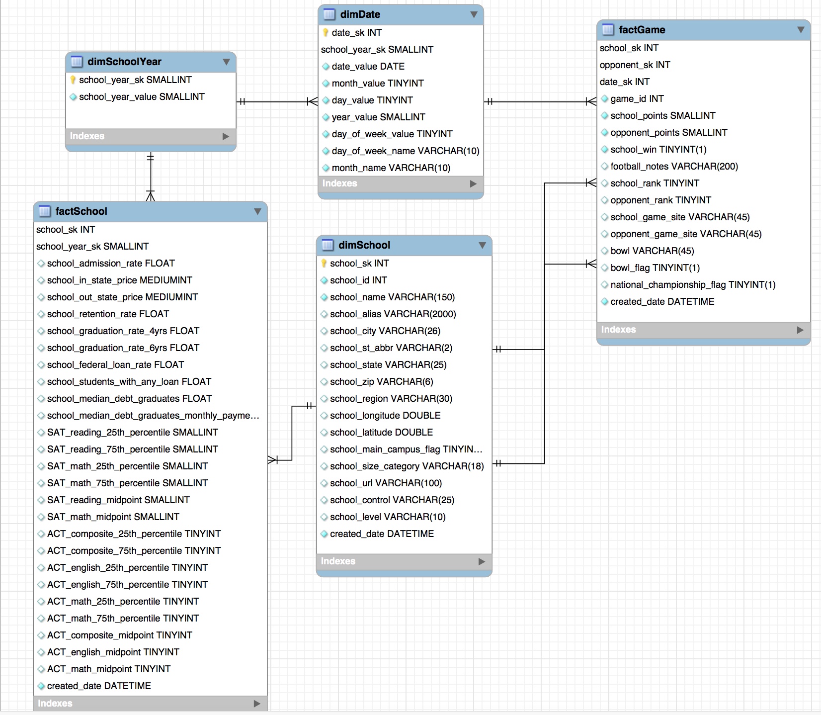
Other challenging aspects of modeling this data are how best to handle the dynamic of dimSchool being a role playing dimension, as well as schools sometimes being winners and sometimes losers. I eventually settled on the solution of loading each game into the factGame table twice, with each role through the perspective of each school playing in that game. I also decided to add in a dimDate attribute of school year, and then snowflake it. I did this in order to better handle the grain discrepancy between the football game data (played on a specific date) and the school data (tied to a school year) when trying to report on the two sets of data at once. Having only the school year in the school data created a many to many relationship and snowflaking this dimension solved that issue.
Here is the final data model created in MySQL Workbench.
Fuzzy Text Matching
As mentioned previously, the only variable that ties the school data and the football data together is the school name. Thus, in order to be able to join the two data sets together, I need to create a lookup table that contains the school name from the football data and the corresponding school name from the school data. I’ll use fuzzy text matching in R to create this table.
I created a function to perform the fuzzy text matching. One benefit of this function is that it allows the user to concatenate text either before or after the football school name prior to the fuzzy matching. This is important because several of the school names from the football data are shortened (e.g Arizona instead of The University of Arizona). This concantenation can improve the fuzzy matching in some cases.
A cross join is used to match up all the football names with all of the school names so each combination can be assessed for string distance. I’m using all available string distance methods in the stringdist function so I can filter the data based on the method(s) that provide the best results. The definitions of the different string distance methods can be found here.
fuzzy_text_matching <- function(x, y, text = NULL, before_after = NULL) {
  # x = transformed school data
  # y = transformed football data
  # get unique school names
  unique_school_names <- x %>%
    filter(school_year_start == max(school_year_start) & school_main_campus_flag == 1) %>%
    select(school_name) %>%
    distinct() %>%
    mutate(dummy = 1) # create dummy variable to join on

  # get unique football school names by combining values in the school and opponent columns into one column
  unique_football_names <- y %>%
    select(school, opponent) %>%
    gather("delete", "football_name", 1:2) %>%
    select(football_name) %>%
    distinct() %>%
    mutate(dummy = 1) # create dummy variable to join on

  # use stringdist for fuzzy text matching; run through all possible methods used for distance calculation
  # cross join football names with all school names (227 football names * 2187 school names = 496449 possible combinations)
  ft_all <- unique_football_names %>%
    mutate(low_football_name = tolower(football_name)) %>%
    inner_join(unique_school_names, by = "dummy") %>% # join on dummy variable to essentially do a cross join
    mutate(low_school_name = tolower(school_name))

  method_list <- c("osa", "lv", "dl", "hamming", "lcs", "qgram", "cosine", "jaccard", "jw", "soundex")
  if (is.null(text) & is.null(before_after)) {
    ft_result <- method_list %>%
      map_dfc(~ tibble(stringdist(ft_all$low_football_name, ft_all$low_school_name, method = .x))) %>%
      set_names(method_list) %>%
      bind_cols(ft_all, .) %>%
      select(-dummy, -low_school_name, -low_football_name)
  } else if (is.null(text) & !is.null(before_after)) {
      stop("Text to concantenate with football name is missing", call. = FALSE)
  } else if (!is.null(text) & is.null(before_after)) {
      stop("Please specify if text should be concantenated before or after the football name", call. = FALSE)
  } else if (!(before_after %in% c("before", "after"))) {
      stop("The 'before_after' argument must have a value of before or after", call. = FALSE)
  } else if (before_after == "before") {
    ft_before <- ft_all %>%
      mutate(text_football_name = paste(tolower(text), low_football_name))
    ft_result <- method_list %>%
      map_dfc(~ tibble(stringdist(ft_before$text_football_name, ft_before$low_school_name, method = .x))) %>%
      set_names(method_list) %>%
      bind_cols(ft_before, .) %>%
      select(-text_football_name, -dummy, -low_school_name, -low_football_name)
  } else {
    ft_after <- ft_all %>%
      mutate(football_name_text = paste(low_football_name, tolower(text)))
    ft_result <- method_list %>%
      map_dfc(~ tibble(stringdist(ft_after$football_name_text, ft_after$low_school_name, method = .x))) %>%
      set_names(method_list) %>%
      bind_cols(ft_after, .) %>%
      select(-football_name_text, -dummy, -low_school_name, -low_football_name)
  }
  return(ft_result)
}
fuzzy_text_res <- fuzzy_text_matching(school_data_transform, football_data_transform)| football_name | school_name | osa | lv | dl | hamming | lcs | qgram | cosine | jaccard | jw | soundex |
|---|---|---|---|---|---|---|---|---|---|---|---|
| Arizona State | University of South Florida-Main Campus | 33 | 33 | 33 | Inf | 38 | 28 | 0.2909866 | 0.5714286 | 0.4581197 | 1 |
| Arizona State | St Petersburg College | 18 | 18 | 18 | Inf | 26 | 20 | 0.5120500 | 0.6250000 | 0.5564713 | 1 |
| Arizona State | Broward College | 12 | 12 | 12 | Inf | 18 | 18 | 0.5449842 | 0.6875000 | 0.5273504 | 1 |
| Arizona State | Luther Rice College & Seminary | 24 | 24 | 24 | Inf | 31 | 25 | 0.4564172 | 0.5000000 | 0.5522589 | 1 |
| Arizona State | State College of Florida-Manatee-Sarasota | 33 | 33 | 33 | Inf | 38 | 30 | 0.1476006 | 0.4705882 | 0.4466996 | 1 |
Now we can filter the data based on the best matches. This is still somewhat of a manual process but the fuzzy text matching is infinitely better than manually matching the strings.
# filter data based on exact matches and results for close matches
text_matches_for_review <- fuzzy_text_res %>%
  filter(jw < 0.20) %>%
  mutate(correct_match = 1) %>% # add column for user to manually update with 0 if the match is no good
  edit()
# this is an iterative process where you can add the correct matches to a final match data table until all schools are matched
fuzzy_text_match_final <- text_matches_for_review %>%
filter(correct_match == 1) %>%
select(football_name, school_name)I also concatenated “university of” to the football school names to see if that improved the text matching for the remaining unmatched schools.
fuzzy_text_conc_before <- fuzzy_text_matching(school_data_transform, football_data_transform, "university of", "before")
# remove the results that have already been matched
fuzzy_text_conc_before <- fuzzy_text_conc_before %>%
  anti_join(fuzzy_text_match_final, by = "football_name")

fuzzy_text_conc_before_review <- fuzzy_text_conc_before %>%
  filter(jw < 0.10) %>%
  mutate(correct_match = 1) %>%
  edit()
# this is an iterative process where you can add the correct matches to a final match data table until all schools are matched
fuzzy_text_match_final <- fuzzy_text_conc_before_review %>%
filter(correct_match == 1) %>%
select(football_name, school_name) %>%
bind_rows(fuzzy_text_match_final)All in all, this process does require iteration, filtering, and manual review. In the end, I was able to match 84% of the school names using the output from the fuzzy text matching. The school names that were difficult to match were ones like penn state = pennsylvania state university-main campus or ucla = university of california-los angeles. Eventually I got a final table that matches each of the football school names with the school names from the school data.
| football_name | school_name |
|---|---|
| Boston College | Boston College |
| Virginia Military Institute | Virginia Military Institute |
| Abilene Christian | Abilene Christian University |
| Alabama A&M | Alabama A & M University |
| Alabama State | Alabama State University |
During this fuzzy text matching process, I found that I was missing the following from the school data: United States Military Academy (Army), United States Naval Academy (Navy), and United States Air Force Academy (Air Force). According to the Scorecard Helpdesk “College Scorecard data are currently limited to institutions that participate in Title-IV federal financial aid programs. As the U.S. service academies do not participate in Title-IV, the data needed for inclusion in Scorecard are unavailable.” So, I made the decision to go directly to The National Center for Education Statistics to get what data I could for these missing schools. I had to export a csv for each year from the website, which is a fairly painful process because the site is a little tricky to figure out. Below, I brought that data into R and transformed it. The different years had different column orders (of course!) in the exported csv files, so that is why I have missing_school_data_1 and missing_school_data_2.
Get Missing Data
get_missing_data <- function(file_path, column_names, column_pos) {
  file_names <- list.files(path = file_path, pattern = "*\\.csv", full.names = TRUE)
  # Merge all school data files
  combined_data <- file_names %>%
    map_dfr(~ fread(.x, skip = 1, header = FALSE, select = column_pos, col.names = column_names), .id = "index") %>%
    as_tibble() %>%
    mutate_at(vars(index), as.integer) %>%
    mutate(file = basename(file_names[index]))
  return(combined_data)
}
missing_school_data_1 <- get_missing_data("~/Documents/DataProjects/football_schools/school_data/column_order1",
c("school_id",
"school_name",
"school_alias",
"school_city",
"zip",
"school_st_abbr",
"school_url",
"school_longitude",
"school_latitude",
"region",
"level",
"control",
"size_category",
"school_graduation_rate_6yrs",
"SAT_reading_25th_percentile",
"SAT_reading_75th_percentile",
"SAT_math_25th_percentile",
"SAT_math_75th_percentile",
"ACT_composite_25th_percentile",
"ACT_composite_75th_percentile",
"ACT_english_25th_percentile",
"ACT_english_75th_percentile",
"ACT_math_25th_percentile",
"ACT_math_75th_percentile",
"school_admission_rate",
"school_retention_rate"), c(1:6, 8:11, 13:15, 22, 25:34, 37:38))
missing_school_data_2 <- get_missing_data("~/Documents/DataProjects/football_schools/school_data/column_order2",
c("school_id",
"school_name",
"school_alias",
"school_city",
"zip",
"school_st_abbr",
"school_url",
"school_longitude",
"school_latitude",
"region",
"level",
"control",
"size_category",
"school_graduation_rate_6yrs",
"school_admission_rate",
"school_retention_rate",
"SAT_reading_25th_percentile",
"SAT_reading_75th_percentile",
"SAT_math_25th_percentile",
"SAT_math_75th_percentile",
"ACT_composite_25th_percentile",
"ACT_composite_75th_percentile",
"ACT_english_25th_percentile",
"ACT_english_75th_percentile",
"ACT_math_25th_percentile",
"ACT_math_75th_percentile"), c(1:6, 8:11, 13:15, 22, 27:28, 32:41))clean_missing_data <- function(missing1, missing2) {
clean_data <- missing1 %>%
bind_rows(missing2) %>%
filter(school_id %in% c(197036, 128328, 164155)) %>%
mutate(school_zip = str_sub(zip, end = 5),
school_region = recode(region,"0" = "US Service school"),
school_level = recode(level,"1" = "4-year"),
school_control = recode(control,"1" = "Public"),
school_size_category = recode(size_category,"2" = "1,000 - 4,999"),
school_state = recode(school_st_abbr,
"CO" = "Colorado",
"NY" = "New York",
"MD" = "Maryland"),
school_year_start = str_sub(file, end = 4),
school_main_campus_flag = 1) %>%
mutate_at(vars(school_graduation_rate_6yrs, school_admission_rate, school_retention_rate), funs(. / 100)) %>%
mutate_at(vars(school_year_start), as.integer) %>%
select(-index, -file, -zip, -region, -level, -control, -size_category)
return(clean_data)
}missing_school_data <- clean_missing_data(missing_school_data_1, missing_school_data_2)Creating Tables in the Data Warehouse
From the data model, I want to create the tables in my data warehouse on AWS. To do this I first connect to my database in MySQL Workbench. Then select Database > Forward Engineer. The wizard guides you through the process and generates the necessary SQL to create the database and tables.
Now that my tables are created, I want to load the clean data into my data warehouse. The first step is to connect to my database in R. I put my username, password, and host information into a .Renviron file so I could access it without putting it my code.
con <- dbConnect(MySQL(),
                 user = Sys.getenv("RDSuser"),
                 password = Sys.getenv("RDSpw"),
                 host = Sys.getenv("RDShost"),
                 dbname = 'FootballSchoolDW')
dimSchool
Now that I have a connection to the database. I can write the data to it. I could setup the dimSchool table as a type 2 slowly changing dimension, but I decided that I did not need a history of the changes from 2011 to 2015. I found that the changes from one year to the next were minor. Thus, I setup the dimSchool dimension as a type I slowly changing dimension. As a result, you’ll notice that I’m only including the school information from the latest school year that I have, which is 2015.
# filter for only 2015 data and only columns needed for dimSchool
dimSchool <- school_data_transform %>%
  semi_join(fuzzy_text_final, by = "school_name") %>%
  bind_rows(missing_school_data) %>%
  filter(school_year_start %in% max(school_year_start)) %>%
  select(school_id,
         school_name,
         school_alias,
         school_city,
         school_st_abbr,
         school_state,
         school_zip,
         school_region,
         school_longitude,
         school_latitude,
         school_main_campus_flag,
         school_size_category,
         school_url,
         school_control,
school_level)| school_id | school_name | school_alias | school_city | school_st_abbr | school_state | school_zip | school_region | school_longitude | school_latitude | school_main_campus_flag | school_size_category | school_url | school_control | school_level |
|---|---|---|---|---|---|---|---|---|---|---|---|---|---|---|
| 137351 | University of South Florida-Main Campus | USF Main Campus |USF Tampa Campus |USF Tampa |USF | Tampa | FL | Florida | 33620 | Southeast | -82.41588 | 28.05665 | 1 | 20,000 and above | www.usf.edu | Public | 4-year |
| 130934 | Delaware State University | NA | Dover | DE | Delaware | 19901 | Mid East | -75.54053 | 39.18717 | 1 | 1,000 - 4,999 | www.desu.edu | Public | 4-year |
| 139940 | Georgia State University | NA | Atlanta | GA | Georgia | 30303 | Southeast | -84.38667 | 33.75270 | 1 | 20,000 and above | www.gsu.edu | Public | 4-year |
| 145637 | University of Illinois at Urbana-Champaign | Illinois|Illinios|Ilinois|Ilinios|Urbana|Champaign|Champagne|Champaign-Urbana|Champagne-Urbana|Urbana-Champaign|Urbana-Champagne|University of Illinois at Urbana|University of Illinois at Champaign|University of Illinois at Champagne|University of Illinois at Champaign-Urbana|University of Illinois at Champagne-Urbana|UIUC|UICU|University of Illinois at UC|University of Illinois at CU | Champaign | IL | Illinois | 61820 | Great Lakes | -88.23031 | 40.10886 | 1 | 20,000 and above | www.illinois.edu/ | Public | 4-year |
| 126614 | University of Colorado Boulder | U of Colorado|Univ of Colorado|University of Colorado|U of CO|Univ of CO|University of CO|Boulder|CU|CU-Boulder|UCB|CUB|Colorado|Colorado University|U of Colo|Univ of Colo|University of Colo|Colo|Buffs|Buffalos|Buffaloes|CU at Boulder|Golden Buffs|University of Colorado at Boulder | Boulder | CO | Colorado | 80309 | Rocky Mountains | -105.26706 | 40.00442 | 1 | 20,000 and above | www.colorado.edu | Public | 4-year |
dbWriteTable(con, name = "dimSchool", value = dimSchool , append = TRUE, row.names = FALSE)dimDate and dimSchoolYear
Before I can load the fact tables, I need to create the dimDate and dimSchoolYear tables and load them into the data warehouse.
create_date_table <- function(start_year) {
  d <- tibble(date_value = seq(mdy(paste0("01/01/", start_year)), by = "day", length.out = 6940),
              date_sk = as.integer(format(date_value, format = "%Y%m%d")),
              school_year_sk = if_else(month(date_value) %in% c(1, 2, 3, 4, 5, 6, 7), as.integer(year(date_value) - 1), as.integer(year(date_value))),
              month_value = month(date_value),
              day_value = day(date_value),
              year_value = year(date_value),
              day_of_week_value = wday(date_value),
              day_of_week_name = wday(date_value, label = TRUE, abbr = FALSE),
              month_name = month(date_value, label = TRUE, abbr = FALSE)) %>%
               select(date_sk, school_year_sk, everything())
  return(d)
}
dimDate <- create_date_table(2011)| date_sk | school_year_sk | date_value | month_value | day_value | year_value | day_of_week_value | day_of_week_name | month_name |
|---|---|---|---|---|---|---|---|---|
| 20110101 | 2010 | 2011-01-01 | 1 | 1 | 2011 | 7 | Saturday | January |
| 20110102 | 2010 | 2011-01-02 | 1 | 2 | 2011 | 1 | Sunday | January |
| 20110103 | 2010 | 2011-01-03 | 1 | 3 | 2011 | 2 | Monday | January |
| 20110104 | 2010 | 2011-01-04 | 1 | 4 | 2011 | 3 | Tuesday | January |
| 20110105 | 2010 | 2011-01-05 | 1 | 5 | 2011 | 4 | Wednesday | January |
dbWriteTable(conn = con, name = 'dimDate', value = dimDate, append = TRUE, row.names = FALSE)create_school_year <- function(dates) {
# x should be dimDate or equivalent
s <- dates %>%
mutate(school_year_value = school_year_sk) %>%
select(school_year_sk, school_year_value) %>%
distinct()
return(s)
}dimSchoolYear <- create_school_year(dimDate)| school_year_sk | school_year_value |
|---|---|
| 2010 | 2010 |
| 2011 | 2011 |
| 2012 | 2012 |
| 2013 | 2013 |
| 2014 | 2014 |
dbWriteTable(conn = con, name = 'dimSchoolYear', value = dimSchoolYear, append = TRUE, row.names = FALSE)factGame
In the game source data, one row represents two schools, both a winner and loser. In the data warehouse I want to represent a game from each school’s perspective. Therefore, I loaded two rows for each game and defined the school columns in the table as ‘school’ and ‘opponent.’ This allowed me to load both the winner and the loser into the same column on two different rows. For analysis, this permitted me to obtain data for both winners and losers by querying just one column, either ‘school’ or ‘opponent’.
create_factGame <- function(football, dates, text_match) {
  # football should be clean, transformed football data
  # dates should be the dimDate table or equivalent
  # text_match should be the final fuzzy text matching data
  # get SKs
  school_opponent_sks <- dbGetQuery(con, "SELECT school_sk, school_name
                                    FROM FootballSchoolDW.dimSchool")

  # create unique game id by concantenating the school year with the original game number
  final_football_data <- football %>%
    left_join(select(dates, date_value, date_sk, school_year_sk), by = c("game_date" = "date_value")) %>%
    unite(game_id, school_year_sk, game_number, sep = "") %>%
    mutate_at(vars(game_id), as.integer) %>%
    left_join(text_match, by = c("school" = "football_name")) %>%
    rename(school_lookup = school_name) %>%
    left_join(school_opponent_sks, by = c("school_lookup" = "school_name")) %>%
    left_join(text_match, by = c("opponent" = "football_name")) %>%
    rename(opponent_lookup = school_name) %>%
    left_join(school_opponent_sks, by = c("opponent_lookup" = "school_name")) %>%
    rename(school_sk = school_sk.x, opponent_sk = school_sk.y)

  if (any(is.na(final_football_data$school_sk))) {
    warning("Some school SKs are NA. Check before loading data into database.", call. = FALSE)
  }
  if (any(is.na(final_football_data$opponent_sk))) {
    warning("Some opponent SKs are NA. Check before loading data into database.", call. = FALSE)
  }

  winner <- final_football_data %>%
    select(school_sk,
           opponent_sk,
           date_sk,
           game_id,
           school_points,
           opponent_points,
           school_win,
           football_notes,
           school_rank,
           opponent_rank,
           school_game_site,
           opponent_game_site,
           bowl,
           bowl_flag,
           national_championship_flag)

  loser <- final_football_data %>%
    select(opponent_sk,
           school_sk,
           date_sk,
           game_id,
           opponent_points,
           school_points,
           opponent_win,
           football_notes,
           opponent_rank,
           school_rank,
           opponent_game_site,
           school_game_site,
           bowl,
           bowl_flag,
           national_championship_flag)

  # I intentionally want to bind these two tibbles together by the column orders
  # specified above so I get a row for the school and a row for the opponent in the final table
  final_football_ordered <- rbindlist(list(winner, loser)) %>%
    as_tibble() %>%
    arrange(game_id)
  return(final_football_ordered)
}
factGame <- create_factGame(football_data_transform, dimDate, fuzzy_text_final)| school_sk | opponent_sk | date_sk | game_id | school_points | opponent_points | school_win | football_notes | school_rank | opponent_rank | school_game_site | opponent_game_site | bowl | bowl_flag | national_championship_flag |
|---|---|---|---|---|---|---|---|---|---|---|---|---|---|---|
| 221 | 106 | 20110901 | 20111 | 48 | 14 | 1 | NA | NA | NA | home | away | NA | 0 | 0 |
| 106 | 221 | 20110901 | 20111 | 14 | 48 | 0 | NA | NA | NA | away | home | NA | 0 | 0 |
| 30 | 17 | 20110901 | 20112 | 32 | 15 | 1 | NA | NA | NA | away | home | NA | 0 | 0 |
| 17 | 30 | 20110901 | 20112 | 15 | 32 | 0 | NA | NA | NA | home | away | NA | 0 | 0 |
| 23 | 49 | 20110901 | 20113 | 21 | 6 | 1 | NA | NA | NA | home | away | NA | 0 | 0 |
dbWriteTable(conn = con, name = 'factGame', value = factGame, append = TRUE, row.names = FALSE)factSchool
Finally, the factSchool table was loaded. The school_year was obtained from the snowflaked dimSchoolYear table, the school_sk was obtained from the dimSchool table.
create_factSchool <- function(school, missing_data, school_year, text_match) {
  # school should be clean, transformed school data
  # missing_data is the missing school data
  # school_year should be the dimSchoolYear table or equivalent
  # text_match should be the final fuzzy text matching data
  # get SKs
  school_sks <- dbGetQuery(con, "SELECT school_sk, school_name
                           FROM FootballSchoolDW.dimSchool")

  final_school_data <- school %>%
    semi_join(text_match, by = "school_name") %>%
    bind_rows(missing_data) %>%
    left_join(school_sks, by = "school_name") %>%
    left_join(school_year, by = c("school_year_start" = "school_year_value")) %>%
    select(school_sk,
           school_year_sk,
           school_admission_rate,
           school_in_state_price,
           school_out_state_price,
           school_retention_rate,
           school_graduation_rate_4yrs,
           school_graduation_rate_6yrs,
           school_federal_loan_rate,
           school_students_with_any_loan,
           school_median_debt_graduates,
           school_median_debt_graduates_monthly_payments,
           SAT_reading_25th_percentile,
           SAT_reading_75th_percentile,
           SAT_math_25th_percentile,
           SAT_math_75th_percentile,
           SAT_reading_midpoint,
           SAT_math_midpoint,
           ACT_composite_25th_percentile,
           ACT_composite_75th_percentile,
           ACT_english_25th_percentile,
           ACT_english_75th_percentile,
           ACT_math_25th_percentile,
           ACT_math_75th_percentile,
           ACT_composite_midpoint,
           ACT_english_midpoint,
           ACT_math_midpoint)

  if (any(is.na(final_school_data$school_sk))) {
    warning("Some school SKs are NA. Check before loading data into database.", call. = FALSE)
  }
  return(final_school_data)
}
factSchool <- create_factSchool(school_data_transform, missing_school_data, dimSchoolYear, fuzzy_text_final)| school_sk | school_year_sk | school_admission_rate | school_in_state_price | school_out_state_price | school_retention_rate | school_graduation_rate_4yrs | school_graduation_rate_6yrs | school_federal_loan_rate | school_students_with_any_loan | school_median_debt_graduates | school_median_debt_graduates_monthly_payments | SAT_reading_25th_percentile | SAT_reading_75th_percentile | SAT_math_25th_percentile | SAT_math_75th_percentile | SAT_reading_midpoint | SAT_math_midpoint | ACT_composite_25th_percentile | ACT_composite_75th_percentile | ACT_english_25th_percentile | ACT_english_75th_percentile | ACT_math_25th_percentile | ACT_math_75th_percentile | ACT_composite_midpoint | ACT_english_midpoint | ACT_math_midpoint |
|---|---|---|---|---|---|---|---|---|---|---|---|---|---|---|---|---|---|---|---|---|---|---|---|---|---|---|
| 7 | 2011 | 0.3805 | 5800 | 14990 | 0.8752 | 0.2488538 | 0.5171 | 0.4489 | 0.8158580 | 17500.0 | NA | 520 | 620 | 540 | 630 | 570 | 585 | 23 | 27 | 22 | 28 | 23 | 27 | 25 | 25 | 25 |
| 8 | 2011 | 0.4265 | 7056 | 15052 | 0.7046 | 0.1853107 | 0.3458 | 0.7559 | 0.9596323 | 28438.5 | NA | 400 | 470 | 400 | 470 | 435 | 435 | 16 | 20 | 15 | 20 | 16 | 19 | 18 | 18 | 18 |
| 9 | 2011 | 0.5183 | 9410 | 27620 | 0.8314 | 0.1754839 | 0.4731 | 0.5446 | 0.6536679 | 18739.5 | NA | 500 | 590 | 500 | 600 | 545 | 550 | 21 | 26 | 21 | 26 | 20 | 26 | 24 | 24 | 23 |
| 16 | 2011 | 0.6759 | 13838 | 27980 | 0.9275 | 0.6605480 | 0.8243 | 0.4289 | 0.9348945 | 19125.0 | NA | 540 | 660 | 690 | 780 | 600 | 735 | 26 | 31 | 26 | 32 | 26 | 33 | 29 | 29 | 30 |
| 6 | 2011 | 0.8694 | 9152 | 30330 | 0.8380 | 0.4008388 | 0.6814 | 0.3470 | 0.9125573 | 17998.0 | NA | 520 | 630 | 540 | 650 | 575 | 595 | 24 | 28 | 23 | 29 | 23 | 29 | 26 | 26 | 26 |
dbWriteTable(conn = con, name = 'factSchool', value = factSchool, append = TRUE, row.names = FALSE)Create View in SQL
Now that all of the data is loaded into the database, I’m going to create a view using SQL that will be used for the analysis/data visualization work. If the dataset were larger, I would consider creating a materialized view, but for this amount of data a regular view will work fine.
CREATE VIEW viewAnalysis AS
SELECT
  ds.school_id,
    ds.school_name,
    ds.school_city,
    ds.school_st_abbr,
    ds.school_state,
    ds.school_zip,
    ds.school_region,
    ds.school_longitude,
    ds.school_latitude,
    ds.school_main_campus_flag,
    ds.school_size_category,
    ds.school_url,
    ds.school_control,
    ds.school_level,
    fs.school_admission_rate,
    fs.school_in_state_price,
    fs.school_out_state_price,
    fs.school_retention_rate,
    fs.school_graduation_rate_4yrs,
    fs.school_graduation_rate_6yrs,
    fs.school_federal_loan_rate,
    fs.school_students_with_any_loan,
    fs.school_median_debt_graduates,
    fs.school_median_debt_graduates_monthly_payments,
    fs.SAT_reading_25th_percentile,
    fs.SAT_reading_75th_percentile,
    fs.SAT_math_25th_percentile,
    fs.SAT_math_75th_percentile,
    fs.SAT_reading_midpoint,
    fs.SAT_math_midpoint,
    fs.ACT_composite_25th_percentile,
    fs.ACT_composite_75th_percentile,
    fs.ACT_english_25th_percentile,
    fs.ACT_english_75th_percentile,
    fs.ACT_math_25th_percentile,
    fs.ACT_math_75th_percentile,
    fs.ACT_composite_midpoint,
    fs.ACT_english_midpoint,
    fs.ACT_math_midpoint,
    sy.school_year_value,
    SUM(fg.school_points) AS school_points,
    SUM(fg.opponent_points) AS opponent_points,
    SUM(fg.school_win) AS school_wins,
    MIN(fg.school_rank) AS min_school_rank,
    MIN(fg.opponent_rank) AS min_opponent_rank,
    SUM(fg.bowl_flag) AS bowl_games,
  SUM(CASE WHEN (fg.bowl_flag = 1 AND fg.school_win = 1)
          THEN 1
      ELSE 0
      END) AS bowl_wins,
    SUM(fg.national_championship_flag) AS national_championship_games,
    SUM(CASE WHEN (fg.national_championship_flag = 1 AND fg.school_win = 1)
          THEN 1
      ELSE 0
      END) AS national_championship_wins,
    SUM(CASE WHEN (fg.school_game_site = 'home' AND fg.school_win = 1)
          THEN 1
          ELSE 0
          END) AS home_wins,
    SUM(CASE WHEN (fg.school_game_site = 'home' AND fg.school_win = 0)
          THEN 1
          ELSE 0
          END) AS home_loses,
    SUM(CASE WHEN (fg.school_game_site = 'home')
          THEN 1
          ELSE 0
          END) AS home_games,
    SUM(CASE WHEN ((fg.school_game_site = 'away' OR fg.school_game_site = 'neutral' ) AND fg.school_win = 1)
          THEN 1
          ELSE 0
          END) AS road_wins,
    SUM(CASE WHEN ((fg.school_game_site = 'away' OR fg.school_game_site = 'neutral' ) AND  fg.school_win = 0)
          THEN 1
          ELSE 0
          END) AS road_loses,
    SUM(CASE WHEN (fg.school_game_site = 'away' OR fg.school_game_site = 'neutral' )
          THEN 1
          ELSE 0
          END) AS road_games,
    SUM(CASE WHEN (fg.opponent_rank IS NOT NULL AND fg.school_win = 1)
          THEN 1
          ELSE 0
          END) AS wins_against_ranked_opponents,
    SUM(CASE WHEN (fg.opponent_rank IS NOT NULL AND fg.school_win = 0)
          THEN 1
          ELSE 0
          END) AS loses_against_ranked_opponent,
    SUM(CASE WHEN (fg.opponent_rank IS NOT NULL)
          THEN 1
      ELSE 0
      END) AS games_against_ranked_opponent,
    SUM(fg.school_points) - SUM(fg.opponent_points) AS point_differential,
    COUNT(*) as total_games
FROM FootballSchoolDW.factGame AS fg
  INNER JOIN FootballSchoolDW.dimSchool AS ds
  ON fg.school_sk = ds.school_sk
  INNER JOIN FootballSchoolDW.dimDate AS dd
  ON dd.date_sk = fg.date_sk
  INNER JOIN FootballSchoolDW.dimSchoolYear AS sy
  ON dd.school_year_sk = sy.school_year_sk
  INNER JOIN FootballSchoolDW.factSchool AS fs
  ON fs.school_sk = ds.school_sk and fs.school_year_sk = sy.school_year_sk
  GROUP BY
    ds.school_id,
    ds.school_name,
    ds.school_city,
    ds.school_st_abbr,
    ds.school_state,
    ds.school_zip,
    ds.school_region,
    ds.school_longitude,
    ds.school_latitude,
    ds.school_main_campus_flag,
    ds.school_size_category,
    ds.school_url,
    ds.school_control,
    ds.school_level,
    fs.school_admission_rate,
    fs.school_in_state_price,
    fs.school_out_state_price,
    fs.school_retention_rate,
    fs.school_graduation_rate_4yrs,
    fs.school_graduation_rate_6yrs,
    fs.school_federal_loan_rate,
    fs.school_students_with_any_loan,
    fs.school_median_debt_graduates,
    fs.school_median_debt_graduates_monthly_payments,
    fs.SAT_reading_25th_percentile,
    fs.SAT_reading_75th_percentile,
    fs.SAT_math_25th_percentile,
    fs.SAT_math_75th_percentile,
    fs.SAT_reading_midpoint,
    fs.SAT_math_midpoint,
    fs.ACT_composite_25th_percentile,
    fs.ACT_composite_75th_percentile,
    fs.ACT_english_25th_percentile,
    fs.ACT_english_75th_percentile,
    fs.ACT_math_25th_percentile,
    fs.ACT_math_75th_percentile,
    fs.ACT_composite_midpoint,
    fs.ACT_english_midpoint,
    fs.ACT_math_midpoint,
    sy.school_year_value
  ORDER BY sy.school_year_value
# disconnect from RDS
dbDisconnect(con)Creating Tableau Dashboard
I am going to start by building a dashboard in Tableau. Maybe if I get ambitious, I’ll build something similar in Shiny. I only have Tableau Public, which can’t connect directly to my database (only the paid version of Tableau allows this). So, I’ll export a CSV file from the view I just created and use that as my Tableau data source.
Users can filter the data based on various fields and then see the corresponding game stats for the filtered list of schools. The user can also select the years they want to view data for and can choose to view the means or medians of the data for the given years selected. A larger view of the dashboard can be found here.